dim. 18 février 2018
Blog
#teaching

$\newcommand{\I}{\mathrm{i}} \newcommand{\E}{\mathrm{e}} \newcommand{\D}{\mathop{}\!\mathrm{d}} \newcommand{\K}[1]{\left|#1\right\rangle}$

This lecture is intended for students of the “Licence de physique”, and in particular to those interested in theoretical physics. (.pdf)

Skyrmion in magnetic nanostructures

Thermodynamics

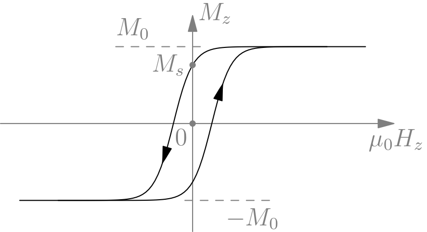
Thermodynamics investigates macroscopic systems in equilibrium. A magnetic material such iron, exhibits a state with definite magnetization at temperatures below the Curie critical temperature (the ferromagnetic state), and a paramagnetic state with vanishing magnetization, above the critical temperature. The equation of state:

$$\boldsymbol{M} = \boldsymbol{M}(T,\boldsymbol{H})$$

relates the magnetization $\boldsymbol{M}$ to the temperature $T$ and the applied magnetic field $\boldsymbol{H}$. A simple form is given by the implicit function:

\begin{equation} \label{mm0} m = m_0\tanh\left(\frac{Jm}{T} + \frac{\mu_B\mu_0 H}{T}\right), \end{equation}

where $m = M/M_s$ is the magnetization in units of its saturation value and in the direction of the applied field, $M_s = M(0,0)$, $m_0$ is the normalized magnetization for infinite field, and, $J$ and $\mu_B$ are two material parameters with units of energy and magnetic moment (Bohr magneton), respectively ($\mu_0$ is the vacuum permeability, and we set the Boltzmann constant to one, $k_B=1$). For $J=0$ and weak magnetic field, $M \sim H/T$ the Curie law for a paramagnet. For zero field $H=0$ and $T<T_c=J$, the implicit equation (\ref{mm0}) has nonvanishing solutions, thus giving an equilibrium finite magnetization, the material is in its ferromagnetic state.

Schematic hysteresis loop of a ferromagnetic material.

Remark: Dimensions of magnetic quantities: magnetic field $[B]=M/eT$, magnetization $[M]=[H]=e/LT$, magnetic moment $[\mu]=[\mu_B]=eL^2/T$, permeability $[\mu_0]=[B/M]= ML/e^2$.

Statistical mechanics

Ferromagnetism is a quantum effect. Form a microscopic point of view, ferromagnetism is the result of the exchange interaction between spins. One simple effective model of this interaction is given by the Heisenberg hamiltonian:

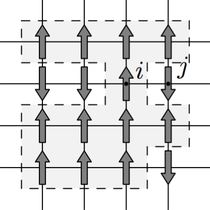
Spins in a square lattice; the gray region is a domain of equally oriented spins

$$\mathcal{H}_\text{ex} = -J\sum_{\langle i,j \rangle} \boldsymbol{S}_i \cdot \boldsymbol{S}_j$$

where $J$ is the exchange coupling constant (we take $\hbar = 1$), and $\boldsymbol{S}_i$ is the spin of site $i$ in the crystal lattice; the sum is over nearest neighbors. The minimum of energy is reached when all spins are aligned, the ferromagnetic state. In fact, equation (\ref{mm0}) is obtained from a mean field approximation of the Heisenberg model, using the tools of statistical physics.

In the framework of the Gibbs canonical ensemble, the free energy $F$ is computed from the partition function $Z$,

$$F(T,\boldsymbol{H}) = -T \ln Z(T,\boldsymbol{H})$$

in the thermodynamic limit. The partition function is a sum over all microscopic energy states of the macroscopic system,

$$Z(T,\boldsymbol{H}) = \sum_{\{\boldsymbol{S}_i\}} \E^{-\mathcal{H}[\boldsymbol{S}_i]/T},$$

where

$$\mathcal{H} = \mathcal{H}_\text{ex} - \mu_B\mu_0 \sum_i \boldsymbol{H} \cdot \boldsymbol{S}_i.$$

contains the interaction between the material spins and the applied field. The probability of a microscopic configuration $S = \{\boldsymbol{S}_i\}$ is,

$$P(S) = \frac{\E^{-\mathcal{H}[S]/T}}{Z}$$

The magnetization is readily computed using the partition function:

$$\boldsymbol M = -\frac{1}{\mu_0 V Z} \frac{\partial }{\partial \boldsymbol{H}}Z = \frac{\mu_B}{V} \sum_i \langle\boldsymbol{S_i}\rangle$$

($V$ is the volume) and the brackets are for the average with the probability $P(S)$. We observe that the macroscopic magnetization is the thermal averaging of the microscopic spins; each spin being associated with an elementary magnetic moment $\mu_B$. Introducing an effective magnetic field:

$$H_\text{eff} = H + \frac{J}{\mu_B\mu_0} \sum_i \langle S_i \rangle$$

(with axes oriented in the direction of the magnetic field), and assuming that the spin can take only two values $S_i = \pm 1/2$, one finds the mean field state equation (\ref{mm0}).

Quantum mechanics

The value of the exchange energy $J$ depends on the electronic structure of the ferromagnetic material; therefore its computation is quantum mechanical, we need to solve the Schrödinger equation to find the matrix element,

$$J = \langle \boldsymbol{x}_1 \boldsymbol{x}_2| U | \boldsymbol{x}_2 \boldsymbol{x}_1\rangle$$

where $U$ is the Coulomb interaction (operator) and $\K{\boldsymbol{x}_1 \boldsymbol{x}_2} = \K{\boldsymbol{x}_1} \otimes \K{\boldsymbol{x}_2}$ is the position two particle state.

Micromagnetics

The Curie temperature of magnetic materials is much larger than the standard normal temperature implying that their natural state is ferromagnetic ($T_c\approx 1000\,\mathrm{K}$ for iron). As such one may think that natural magnets must posses a magnetization of the order of $M_s$, the saturation value at low temperature and magnetic field. However, natural materials are not strongly magnetized. The absence of spontaneous magnetization is due to the existence of magnetic domains. Natural ferromagnets are composed by regions where the magnetization is uniform, but each one may have a different magnetization direction. In a celebrated paper Landau and Lifshitz, developed a theory of these micromagnetic domains.

Micromagnetic theory describes scales intermediate between the microscopic scales of the Heisenberg model, and the macroscopic scales of the thermodynamic model. At these scales, the characteristic length of the magnetization gradients are much larger than the atomic scale (the crystal cell size $a$), and a continuum approximation (or coarse-graining) of the microscopic Heisenberg model becomes relevant. The idea of coarse-graining is to take a bunch of spins of size $\ell$ around a point $\boldsymbol{x}$ and define a local magnetization by the formula,

$$\boldsymbol{M}(\boldsymbol{x},t) \sim \frac{1}{V(\ell)} \sum_{i\in B_\boldsymbol{x}(\ell)} \langle \boldsymbol{S}_i(t) \rangle$$

where $B_\boldsymbol{x}(\ell)$ is a ball of radius $\ell$ and center $\boldsymbol{x}$, $V(\ell)$ is its volume, and where $t$ accounts for the time variation, due to the presence of an external time dependent field, or more generally, to the evolution of a non-equilibrium state. The coarse-grained magnetization is called the order parameter of the magnetic material within the Landau theory of phase transition, and can be used in a form equivalent to the hydrodynamics quantities, such the velocity field or the pressure of a fluid.

In the continuum limit the magnetic hamiltonien becomes a free energy depending on the order parameter $F[\boldsymbol{M}]$ whose minimization gives the evolution equation of the magnetization. For instance, near the ferromagnetic-paramagnetic transition, the mean field behavior (we used in the thermodynamic section), is essentially recovered with the Landau free energy:

$$F(M,H) = F_0(T) + a(T) M^2 + b M^4 - \mu_0 M H$$

where $a,b$ are phenomenological coefficient, which can be deduced from a microscopic calculation, and, near the transition $a\sim T - T_c$ change sign. The Landau free energy can be easily generalized to take into account spatial inhomogeneities and temporal variation of the order parameter.

The Heisenberg part of the magnetic Landau free energy is,

$$F_\text{ex} = \int_V \D V\, A |\nabla \boldsymbol M|^2,$$

where $A \sim J/aM_s^2$ is the exchange parameter, related to $J$. This exchange term can be completed with other terms taking into account the magnetic anisotropy, the spin orbit coupling (Dzyaloshinskii-Moryia) or the magnetic dipole energy.

The general form of the Landau-Lifshitz equation is,

\begin{equation} \label{LL} \frac{\partial }{\partial t} \boldsymbol{m} = -\frac{\gamma}{M_s} \boldsymbol{m} \times \frac{\delta F }{\delta \boldsymbol{m}} \end{equation}

written in terms of the normalized magnetization $\boldsymbol{m} = \boldsymbol{M}/M_s$, and ensuring that the norm $|\boldsymbol{m}| = 1$ is conserved. Here, $\gamma$ is the gyromagnetic ratio (it has units of charge over mass, $e/M$), which gives the characteristic time scale $\tau_0 = \mu_0 M_s/\gamma$. Using for the free energy the exchange term, one obtains,

$$ \frac{\partial }{\partial t} \boldsymbol{m} = \kappa \boldsymbol{m} \times \nabla^2 \boldsymbol{m}, \quad \kappa = 2\gamma A M_s$$

where $\kappa$ is a parameter with the dimensions $L^2/T$ (angular momentum per unit mass). The Landau-Lifshitz equation is reminiscent of the Euler equation describing the rotation of a rigid body rotation:

$$\frac{\D \boldsymbol{L}}{\D t} = \boldsymbol{L} \times \boldsymbol{\omega},$$

to which one may add the applied torques; where $\boldsymbol{L}$ is the angular momentum and $\boldsymbol{\omega}$ the rotation frequency.

Our goal now is to find explicit solutions of the Landau-Lifshitz equation in the case of magnetic films: almost two dimensional layers of magnetic material deposited on a substrate. The motivation to study thin films is provided by the experimental discovery of a skyrmion lattice phase in MnSi. Skyrmions phases were found in other chiral metals, and insulating magnetic films.

A skyrmion is a helical arrangement of spins, with a central core pointing up, say, inside a region of uniform down magnetization (figure below). The whole magnetization texture covers all space directions (solid angle swept by $\boldsymbol{m}$ is $4\pi$). In a real material the skyrmions are stabilized by a weak magnetic field, spin-orbit coupling or anisotropy, here we shall neglect these effects to concentrate in the topology of the magnetic texture, which depends essentially on the exchange interaction.

Stereographic projection: each point of the spher (or equivalently each orientation $\boldsymbol{n}$) is mapped to a point in the complex plane ($z = x + \I y$).

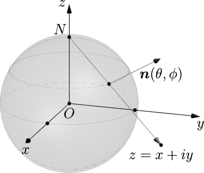
It is convenient to map the magnetization defined on the Bloch sphere, to a complex function $w = w(z)$, with $z = x + \I y$. The stereographic projection of the unit vector on the sphere $\boldsymbol{m} = (\sin\theta \cos\phi, \sin\theta \sin\phi, \cos\theta)$ to the complex plane $w = \mathrm{Re}\, w + \I \mathrm{Im}\, w$ is given by,

$$w = \frac{m_x+\I m_y}{1+m_z} = \tan \frac{\theta}{2} \E^{\I \phi}\,,$$

which gives the inverse relations,

$$m_x = \frac{w+\bar{w}}{1+|w|^2}\,,\; m_y = \frac{1}{\I} \frac{w-\bar{w}}{1+|w|^2}\,,\; m_z = \frac{1-|w|^2}{1+|w|^2}\,,$$

where the over bar represents complex conjugation. The Landau-Lifshitz equation in the new function $w$, becomes:

$$\I \partial_t w = -\kappa\partial \bar{\partial} w + \frac{2 \kappa \bar{w}}{1+|w|^2} \partial w \bar{\partial} w$$

where $\partial=\partial/\partial z=(\partial/\partial x- \I \partial/\partial y)/2$. One immediately observes that any harmonic function is a stationary solution (Belavin and Poliakov, 1975):

$$\bar{\partial} w(z) = 0\,.$$

The physical relevant solutions are those that minimize the total energy. One of such solutions is the trivial $w = 0$, corresponding to a uniform magnetization (the ferromagnetic state), which has vanishing energy. Other finite energy solution can be obtained by noting that the Landau-Lifshitz equation conserves the topological charge:

$$Q = \int \frac{\D\boldsymbol x}{4\pi} \boldsymbol m\cdot\partial_x\boldsymbol m\times \partial_y \boldsymbol m\,.$$

By putting the integral in spherical coordinates,

$$Q=\frac{1}{4\pi}\int \D \theta(\boldsymbol x) \D \phi(\boldsymbol x) \sin\theta(\boldsymbol x)$$

we find that $Q$ is related to the number of times that the magnetic texture covers the solid angle $4\pi$; $Q$ only depends on the topology of the vector field $\boldsymbol{m}$. In the stereographic projection, the topological charge reads,

$$Q = \int \frac{\D x \D y}{\pi} \frac{|\partial w|^2 - |\bar \partial w|^2}{(1+|w|^2)^2}\,.$$

The energy (per unit height of the film), in the same variables is,

$$E = 4A M_s^2\int \D x \D y \frac{|\partial w|^2 + |\bar \partial w|^2}{(1+|w|^2)^2}\,.$$

Comparing the $Q$ and $E$ equations for harmonic $w$, we find the relation,

$$E = 4\pi AM_s^2 Q\,,$$

showing that analytic functions give a finite energy, depending only on their topological charge. This charge will be given by the number of zeros and poles of the analytic function $w = w(z)$.

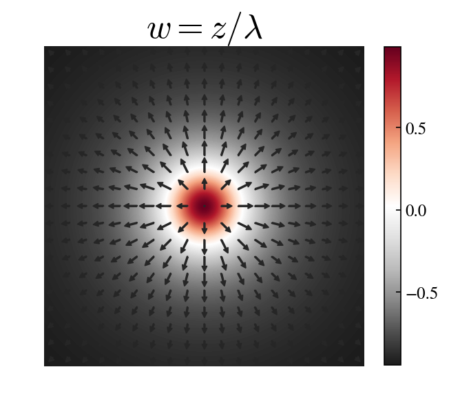
Isolated skyrmion and skyrmion lattice, obtained from two different choices of $w = w(z)$, the stereographic representation of the unit magnetization vector. The arrows are the projection of the magnetization vector on the plane $(x,y)$, and the colors map the $z$-component of the spin (one at the center, and minus one at infinity).

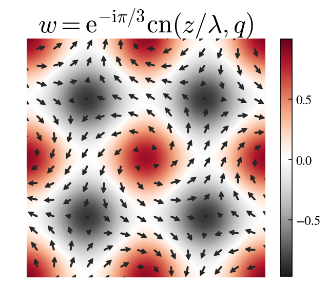
The simplest nontrivial solution is then a polynomial with a single zero, representing an isolated skyrmion,

$$w(z) = \frac{z}{\lambda}$$

where the parameter $\lambda$ fixes the size of the skyrmion: once mapped onto the sphere it has a pure radial distribution (hedgehog). A more complex texture is obtained using the elliptic Jacobi functions, to represent a lattice of skyrmions,

$$w(z) = \E^{-\I \alpha}\mathrm{cn}(z/\lambda, q),$$

of parameters $\alpha = \pi/3$ and $q = 1/2$, we plotted in the above figure.

Applications

Nanometric magnetic structures like skyrmions are good candidates to create ultradense memories (Fert et al. 2013), and other spintronic devices (Rosch, 2016). To achieve such goal it is important to find physical effects allowing the manipulation of skyrmions to control their nucleation, destruction and motion. One possibility is to interact with the skyrmion through a spin polarized current: the itinerant spins can exerce a torque on the fixed magnetization, and hence change their orientation. This effect was discovered by Slonczewski in 1996 and is called the spin transfer torque.

Another possibility is to build heterostructures with a layer of a topological insulator in contact with a magnetic film, to manipulate the skyrmion using electric fields. A topological insulator is a bulk insulator that supports spin polarized conducting channels at their surface; this effect is related to the topology of the electronic bands, which in a topological insulator are inverted (the valence band is above the conducting one, separated by a large gap), combined with a strong spin-orbit coupling. In these heterostructures, one can use the magnetoelectric effect, intrinsic in three dimensional topological insulators, to interact with the skyrmion. Under the influence of the helical electronic modes of the surface polarized currents, a charge is induced in the skyrmion, which then can be displaced by an electric field.