$\newcommand{\I}{\mathrm{i}} \newcommand{\E}{\mathrm{e}} \newcommand{\D}{\mathop{}\!\mathrm{d}} \newcommand{\Di}[1]{\mathop{}\!\mathrm{d}#1\,} \newcommand{\Dd}[1]{\frac{\mathop{}\!\mathrm{d}}{\mathop{}\!\mathrm{d}#1}} \newcommand{\bra}[1]{\langle{#1}|} \newcommand{\ket}[1]{|{#1}\rangle} \newcommand{\braket}[1]{\langle{#1}\rangle}$

Lectures on statistical mechanics.

Gibbs ensembles

The main idea of statistical mechanics, as formulated by Boltzmann and Gibbs, is to describe the microscopic state of equilibrium systems in terms of the probability of an ensemble of configurations compatible with the thermodynamic variables of the macroscopic state. Gibbs devised a set of identical thermodynamic systems differing in their microscopic state, and associated to this set a probability measure; in fact, it is enough to replace the set of systems by an ensemble of macroscopic subsystems. The probability depends on both the microscopic hamiltonian and the state variables. In contrast to Gibbs theory of equilibrium systems, Boltzmann focused on the mechanical description of a macroscopic system and its approach to equilibrium, a kinetic point of view.

Boltzmann fundamental insight was his identification of the combinatorial entropy, a measure of the microstates information bearing, with the thermodynamic entropy. The content of information is proportional to the number of microstates matching the same macrostate. In quantum mechanics this number is well defined, and related to the number of energy levels, spin polarizations, and other quantum numbers. In classical mechanics one must assume (using a semiclassical limit) that the number of microstates is proportional to the volume they occupy in phase space, normalized by the quantum action $\hbar$.

Boltzmann

The extensive thermodynamic variables characterizing the macrostate are the energy $E$, the volume $V$ and the number of particles $N$ (generalization to other extensive variables is straightforward). An equilibrium isolated system of fixed volume and particle number is in a thermodynamic state that depends only on its energy; the set of microstates compatible with a macroscopic energy is the microcanonical ensemble. The energy spectrum of a confined quantum system is discrete but it tends to a continuum in the thermodynamic limit,

$$N \rightarrow \infty,\; V \rightarrow \infty, \quad \mbox{such that}\quad N/V \rightarrow \mbox{const.}$$

the spacing of the energy levels $\Delta E$ is exponentially small in the number of particles $N$:

$$\Delta E \sim \E^{-N}.$$

One may understand this order of magnitude from the fact that the number of energy levels of a quantum system growth exponentially with the number of particles (i.e with the dimension of the hilbert space). This means that the macroscopic energy of the system is compatible with a huge number of microscopic energy levels: for large $N$ one cannot distinguish between neighboring levels.

Therefore, the macroscopic value of the energy $E$ is compatible with microscopic energy levels $E_n$ ($n\in \mathbb{N}$) in the interval

$$E_n \in [E, E+\Delta]$$

where $\Delta$ is small but macroscopic $\Delta/E \ll 1$, one may consider that, in the thermodynamic limit, $\Delta/E \rightarrow 0$. (This is effectively the case if, following the central limit theorem, $\Delta$ represents the strength of the energy fluctuations around the mean value $\Delta \sim \sqrt{N}$.) More importantly, the quantum state of a macroscopic system,

$$\rho = \sum_n P_n \ket{n}\bra{n}, \quad \sum_n P_n = 1$$

where $\ket{n}$ are the eigenvectors of the system’s hamiltonian $H\ket{n} = E_n \ket{n}$, is generally not an eigenstate of $H$. Indeed, in principle the $P_n$ are arbitrary, depending for instance on the preparation of the system. Consequently, a macroscopic fraction of the set of energy states $E_n$ contributes to a state with thermodynamic energy $E$.

The fundamental statistical hypothesis formulated by Boltzmann (applied to a general quantum system), is that the microstate probabilities are a priori equal:

$$P(E_n) = \begin{cases} \frac{1}{\Omega_\Delta(E)} & \text{if } E<E_n<E + \Delta\\ 0 & \text{otherwise}\end{cases}$$

where

$$\Omega_\Delta(E) = \#\{E_n, E_n \in [E, E + \Delta]\}$$

is the number of states in the energy band of width $\Delta$.

If we denote $\Omega(E)$ the total number of states having energies below $E$, $E_n < E$:

$$\Omega_\Delta(E) = \Omega(E+\Delta) - \Omega(E) \approx \frac{\partial \Omega(E)}{\partial E} \Delta \equiv \nu(E) \Delta$$

where

$$\nu(E) = \frac{\partial \Omega(E)}{\partial E}$$

is the density of states.

The Boltzmann entropy of such a system is given by his famous formula,

$$S = k_{\mathrm{B}} \ln \Omega(E)$$

where $k_{\mathrm{B}} = 1.3806\,4852\,10^{-23}\,\mathrm{JK^{-1}}=1$ is the Boltzmann constant (the last identity is a definition of the kelvin in energy units).

It is worth noting that, in the thermodynamic limit, the Boltzmann entropy and therefore the other thermodynamic properties of the system, do not depend on the subextensive parameter $\Delta \ll E$ (for instance $\Delta \sim \mathcal{O}(N^{1/2}$). Indeed,

$$\ln \Omega_\Delta = \ln \Omega + \mathcal{O}\left( \ln \frac{E}{N\Delta} \right)\,.$$

For example, if we take a system of $N$ free particles, the number of states inside a sphere of radius (in wavenumber space) $K \sim \sqrt{E}$ and dimension $N$ is essentially concentrated on its surface: $\ln \Omega \sim \ln K^N \sim \ln K^{N-1}$ (for $N \rightarrow \infty$).

The Boltzmann formula can easily be deduced from the general expression of the quantum von Neumann entropy:

$$S = - \mathrm{Tr}\, \rho \ln \rho\,,$$

using the hypothesis of a priori equal probabilities, given by $P(E_n)$ above. It is interesting to note that the number of states,

$$\Omega(E) = \E^{S(E)} \rightarrow \E^{N s(E/N)}$$

is effectively exponentially large in the thermodynamic limit, as a consequence of the extensivity of the entropy; here $s$ is the entropy density (per particle). The typical separation $D$ of levels in the band of width $\Delta$ is then of the order of $D(E) \sim \Delta \E^{-N s(E/N)}$.

In summary, the microcanonical distribution of microstates probabilities is

\begin{equation} \label{e:micro} \rho(E) = \frac{\delta(E-H)}{\nu(E)} \,, \quad \nu(E) = \mathrm{Tr}\, \delta(E-H) \end{equation}

in terms of the hamiltonian operator $H$ and the thermodynamic energy $E$ of an isolated quantum system; $\nu(E)$ is the density of states ($\nu(E) \sim \Omega_\Delta(E)/\Delta$).

The microcanonical ensemble describes isolated systems in terms of their energy; a more general situation is that of a subsystem exchanging energy with a large system at fixed temperature; the set of the corresponding microstates is the canonical ensemble.

Let the system’s hamiltonian $H_S = H + H_R$ be split into a subsystem part $H$ and a “reservoir” part $H_R$; the density operator of the subsystem $\rho$ is obtained by the partial trace of the total system $\rho_S$ on the reservoir degrees of freedom:

$$\rho = \mathrm{Tr}_R \, \rho_S = \frac{\mathrm{Tr}_R \, \delta(H + H_R - E_S)}{\mathrm{Tr}_S \, \delta(H_S - E_S)} = \frac{\nu_R(E_S-H)}{\nu_S(E_S)}\,,$$

where we used that the partial trace over the bath of the total state $\rho = \delta(E-H)/\nu(E)$ is EX,

$$\mathrm{Tr}_R \delta(H_S-E_S) = \nu_R(E_S - H),$$

the number of states of the reservoir with energies near the energy of the subsystem. If $E$ is the typical energy of the subsystem, we have $E \ll E_S$, and we can then expand the logarithm of $\Omega$, which is the entropy, to obtain:

$$\nu_R(E_S-H) \approx \nu_R(E_S)\, \E^{-H/T},\quad \frac{1}{T} = \frac{\D S(E_S)}{\D E_S}$$

where we defined the temperature $T$ of the total system. Indeed, for any eigenvalue $E_n$ of $H$ we have,

$$\nu_R(E_S-E_n) = \frac{\exp[S_R(E_S-E_n)]}{\Delta_S} \approx \frac{1}{\Delta_S} \exp\left[ S_R(E_S) - \frac{\D S_R(E_S)}{\D E_S} E_n \right]\,,$$

which readily leads to the above expression ($\Delta_S$ is the energy band width of the corresponding microcanonical distribution of the entire system). The reservoir temperature is obviously equal to the total system temperature. Note that as a consequence of the large size limit of the reservoir, the last formula only involves quantities related to the subsystem, the reservoir enters through the temperature.

The density operator of the canonical ensemble is

\begin{equation} \label{e:canon} \rho(T,V) = \frac{\E^{-H/T}}{Z}, \quad Z(T,V) = \mathrm{Tr} \, \E^{-H/T} \end{equation}

where $H$ is the hamiltonian of a quantum system of volume $V$ in contact with a reservoir at temperature $T$; $Z=Z(T,V)$ is the partition function.

More generally, a subsystem can exchange with its surroundings not only energy at fixed temperature, but also particles at fixed chemical potential:

$$\frac{1}{T} = \left. \frac{\partial S}{\partial E}\right|_{(N,V)}\,,\quad \mu = -T \left. \frac{\partial S}{\partial N}\right|_{(E,V)}$$

the corresponding ensemble calls grand canonical, and it is particularly useful for actual computations of statistical models. Adding the number of particles as a new variable $S=S(E,N)$ (with fixed volume), a similar reasoning as the one used to obtain the canonical distribution, leads to the

grand canonical density operator,

\begin{equation} \label{e:grand} \rho(T,\mu,V) = \frac{\E^{-(H - \mu \hat{N})/T}}{Z}, \quad Z(T,\mu,V) = \mathrm{Tr} \, \E^{-(H-\mu N)/T} \end{equation}

where $\hat{N}$ is the number operator and $\mu$ the chemical potential.

If the spectrum of $\hat{N}$ is the set of natural numbers $N=0,1,2,\ldots$ and $\hat{N}$ commutes with $H$, we can write the grand canonical partition function as a power series in the fugacity $z=\E^{\mu/T}$:

\begin{equation} \label{e:grandsum} Z(T,\mu,V) = \sum_{N=0}^\infty z^N \mathrm{Tr}\, \E^{-H_N/T} = \sum_{N=0}^\infty z^N Z_N(T,V) \end{equation}

where $Z_N(T,V)$ is the canonical partition function of $N$ particles with hamiltonian $H_N$. In the same way as the exchange of energy between subsystems of an equilibrium system must satisfy the conservation of the total energy, condition that implies the equality of the temperatures, the exchange of particles at equilibrium implies the equality of chemical potentials. In contrast, for a system that do not conserve the number of particles, such as the photons in a cavity (photons are emitted and absorbed by the walls), the chemical potential must vanish $\mu=0$. Indeed, if the number of particles is variable, at equilibrium the free energy $F(T,N)$ is minimal: the condition $(\partial F/\partial N)_{(T,V)} = \mu = 0$ specifies its equilibrium value.

Remark that in the thermodynamic limit the number of particles and volume tend to infinity, stressing the fact that at thermodynamic equilibrium the physical properties cannot depend on the exact number of particles: isolated, closed systems that exchange energy, or open systems that can also exchange particles, are in this limit equivalent. The Gibbs ensembles, microcanonical, canonical or grand canonical, are therefore equivalent.

The corresponding ensembles for a classical system of $N$ particles are obtained from the quantum ones by replacing the trace by an integral over the phase space $\Gamma$,

$$\mathrm{Tr} \rightarrow \frac{1}{N!}\int_\Gamma \prod_{n=1}^N \frac{\D \boldsymbol x_n \D \boldsymbol p_n}{(2\pi\hbar)^3}$$

and considering the hamiltonian as a function over the phase space. The factor $1/N!$ takes into account the identity of particles (a quantum effect). Note however that the validity of the classical formulas is difficult to assess, and must be verified for each model. For instance, free particles of mass $m$ at temperature $T$ and density $n=N/V$ can be characterized by the nondimensional parameter

$$g = n \lambda_T^3\,,\quad \lambda_T = \sqrt{\frac{2\pi\hbar^2}{mT}}$$

which compares the thermal de Broglie length $\lambda_T$ to the mean distance between particles $n^{-1/3}$; when $g \gg 1$ quantum effects become important: this is the case for dense or low temperature systems (“degenerate” fermi and bose gases). For oscillator systems of typical frequency $\omega$, one may define the parameter $g = \hbar \omega/T$ which separates the quantum ($g \gg 1$) and classical regimes ($g \ll 1$) (vibrations and rotation of molecules).

Thermodynamics

The knowledge of the partition function allows the computation of the thermodynamics properties of statistical systems. For instance, in the microcanonical ensemble $\Omega$ gives the entropy $S=S(E,N,V)$ from which one deduces the temperature and chemical potential (see the formulas above), as well as the pressure:

$$P = T \left. \frac{\partial S}{\partial V}\right|_{E,N}\,.$$

The canonical partition function $Z(T,N,V)$, for a fixed number of particles $N$, is related to the Helmholtz free energy $F$ by,

$$F(T,V) = -T \ln Z(T,N,V) = E - TS\,,$$

and the grand canonical partition function $Z(T,\mu,V)$ with the thermodynamic potential $\Phi$:

$$\Phi(T,\mu,V) = -T \ln Z(T,\mu,V) = E - TS - \mu N = -PV\,.$$

The dependency on the volume $V$ is through the Hamiltonian: a variation $\D V$ of the volume leads to a variation of the hamiltonian spectrum $\D H$; their ratio gives the pressure:

$$P = - \left\langle \frac{\partial H}{\partial V} \right\rangle\,.$$

More generally, the variation of the free energy as a function of $(T,N,V)$, is,

$$\D F(T,N,V) = -S \D T + \mu \D N - P \D V$$

which gives the entropy, chemical potential and pressure by the partial derivatives:

$$S = - \frac{\partial F}{\partial T}\,,\quad \mu = \frac{\partial F}{\partial N}\,,\quad P = - \frac{\partial F}{\partial V}\,.$$

Similar expressions can be obtained from the variation of the grand potential $\D \Phi = -S\D T - N \D \mu - P \D V$:

$$S = - \frac{\partial \Phi}{\partial T}\,,\quad N = -\frac{\partial \Phi}{\partial \mu}\,,\quad P = - \frac{\partial \Phi}{\partial V} = - \frac{\Phi}{V}\,.$$

The two last equations $N = N(T,\mu,V)$ and $P = P(T,\mu,V)$ determine the equation of state $P = P(T,N,V)$, after elimination of the chemical potential.

Second partial derivatives of the free energy (or the partition function) are related to the fluctuations of thermodynamic quantities; for example, taking the derivative of $F/T$:

$$-\frac{\partial \ln Z}{\partial \frac{1}{T} } = \frac{1}{Z} \mathrm{Tr}\, H \E^{-H/T} = \braket{H} = E$$

we obtain,

$$E = \frac{ \partial \frac{F}{T} }{ \partial \frac{1}{T} }\,;$$

and taking now the second derivative,

$$C_V = \frac{\partial E}{\partial T}\,,$$

which is the heat capacity at constant volume EX,

$$C_V = \frac{1}{T^2} \frac{\partial^2 \ln Z}{\partial \left(\frac{1}{T}\right)^2 } = \frac{\braket{H^2} - \braket{H}^2}{T^2} = \left(\frac{\Delta E}{T}\right)^2$$

we get the desired relation to the energy fluctuations (in the canonical ensemble). This type of relation between the variation of an intensive quantity, here the temperature, and the response of the system, here a variation of the energy ($\Delta E = C_V \Delta T$), is one example of a fluctuation-response relation. The proportionality coefficient, the heat capacity, is what is called a susceptibility; other examples are the coefficients of thermal dilatation, compressibility, and the magnetic susceptibility.

More generally, examples of linear relations between an applied field and the response of the system near thermodynamic equilibrium, are the transport coefficients like diffusion, electric or heat conductivities, and viscosity, related respectively, to the fluctuations of concentration, electric or heat currents, and momentum gradients.

Applications

A system of oscillators

As an example of the use of the microcanonical ensemble, we consider a set of $N$ harmonic oscillators, with hamiltonian,

$$H = \sum_{x=1}^N \hbar \omega (a^\dagger_x a_x + 1/2)$$

frequency $\omega$ (we take $\hbar=\omega=1$, such that the energy unit is $\hbar\omega$), and $a_x$ the annihilation operator of the oscillator $x$. We may think that $x$ represent the position in a one dimensional lattice. The oscillators are independent, interactions can be added in a second step: for example considering that the positions in the lattice are themselves oscillators.

The density of states $\nu(E) = \mathrm{Tr}\,\delta(E-H)$ is readily obtained form the spectrum

$$E_{n_x} = n_x + 1/2, \quad n_x=0,1,\ldots\,; \; x=1,2,\ldots,N\,,$$

of each oscillator,

$$\nu(E) = \sum_{n_1} \ldots \sum_{n_N} \delta\left(E-\sum_x (n_x + 1/2)\right)$$

and using the representation

$$\delta(x) = \int_{-\infty}^\infty \frac{\D k}{2\pi} \E^{\I k x}$$

of the Dirac delta function:

$$\nu(E) = \sum_{n_1} \ldots \sum_{n_N} \int_{-\infty}^\infty \frac{\D k}{2\pi} \exp\left[ \I k \left(E-\sum_x (n_x + 1/2)\right) \right]\,.$$

The summation over $n_x$ are power series of the form

$$\sum_{n=0}^\infty x^n = \frac{1}{1-x}\,;$$

using this relation the integrands factorize:

$$\nu(E) = \int_{-\infty}^\infty \frac{\D k}{2\pi} \E^{\I k (E-N/2)} \prod_x \frac{1}{1-\E^{-\I k}}$$

that, after rearranging the exponentials, can be written as,

$$\nu(E) = \int_{-\infty}^\infty \frac{\D k}{2\pi} \E^{N f(k)}\,,\quad f(k) = \I \epsilon k - \ln(2 \I \sin(k/2))$$

where $\epsilon = E/N$. The asymptotic value, for large $N$, of this integral can be evaluated using the Laplace method:

$$\int_{-\infty}^\infty \D k \, \E^{N f(k)} \approx \sqrt{\frac{2\pi}{-f''(k_0) N}} \E^{N f(k_0)}\,,\quad f'(k_0)=0\,.$$

The idea is that the main contribution to the convergent integral comes from the maximum value of the integrand (or in the case of an oscillating function, to its slower oscillation); values away from the stationnary points of $f(k)$ decrease exponentially fast with the large parameter $N$ (or cancels if rapidly oscillating). Then the computation of the integral reduces to its value at the extrema of $f$ (at point $k_0$) and the gaussian integral around this minimum. Therefore, we must compute the value $k_0$ for which $f'(k) = 0$.

We use sympy to compute the minimum of $f(k)$ EX:

from sympy import *
init_printing()
k, epsilon, x = symbols("k, epsilon, x", real = True)
f = I*epsilon*k - ln(2*I*sin(k/2)) # function definition
f

$$\I \epsilon k - \ln{\left (2 \I \sin{\left (\frac{k}{2} \right )} \right )}$$

df = simplify(diff(f, k)) # derivative
df

$$\I \epsilon - \frac{1}{2 \tan{\left (\frac{k}{2} \right )}}$$

solve by substitution of $\exp(\I k/2) \rightarrow x$, this transforms the trigonometric functions in $k$ into rational expressions in $x$, easier to solve; once the solution obtained we put $-2\I \ln(x) \rightarrow k$:

fx = (df.rewrite(exp)).subs(exp(I*k/2), x)
fx

$$\I \epsilon + \frac{\I \left(x + \frac{1}{x}\right)}{2 \left(- x + \frac{1}{x}\right)}$$

solx = solve(fx, x)
solx

$$\left [ - \sqrt{\frac{2 \epsilon + 1}{2 \epsilon - 1}}, \quad \sqrt{\frac{2 \epsilon + 1}{2 \epsilon - 1}}\right ]$$

k_0 = (1/I)*logcombine(2*expand_log(log(solx[1]), force=True), force=True)
k_0

$$- \I \ln{\left (\frac{2 \epsilon + 1}{2 \epsilon - 1} \right )}$$

w = Wild("w") # any expression
s = collect(expand(expand_log(
    simplify((f.subs(k, k_0)).rewrite(exp)), # log(prod) = sum(log)
    force=True)), log(w)) # collect log of any expression
s

$$\left(- \epsilon + \frac{1}{2}\right) \ln{\left (2 \epsilon - 1 \right )} + \left(\epsilon + \frac{1}{2}\right) \ln{\left (2 \epsilon + 1 \right )} - \ln{\left (2 \right )}$$

We finally obtain

$$f(k_0) = \left(\epsilon + \frac{1}{2}\right)\ln\left(\epsilon + \frac{1}{2}\right) - \left(\epsilon - \frac{1}{2}\right) \ln\left(\epsilon - \frac{1}{2}\right)\,,$$

which readily gives, at the leading order, the density of states (neglecting the $O(N^{-1/2})$ non extensive corrections, appearing in the dimensional prefactor of the exponential):

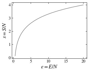
$$\nu(E) \sim \E^{Ns(E/N)}\,,\quad s(\epsilon) = \left(\frac{\epsilon}{\hbar \omega} + \frac{1}{2}\right)\ln\left(\frac{\epsilon}{\hbar \omega} + \frac{1}{2}\right) - \left(\frac{\epsilon}{\hbar \omega} - \frac{1}{2}\right) \ln\left(\frac{\epsilon}{\hbar \omega} - \frac{1}{2}\right)\,,$$

where $S = N s(E/N)$ is the entropy of the system (in the original units).

The entropy of the oscillators system is a monotonic increasing concave function of the energy and vanishes at zero energy (which corresponds to zero temperature).

This formal demonstration, which allowed us to derive the entropy in the microcanonical ensemble of a set of harmonic oscillators masks somewhat the combinatorial, and then probabilistic, nature of the entropy. In fact, we can count the number of quantum states with energy $E$ and then directly compute the entropy $S=\ln \Omega$. Noting that

$$E = \sum_{x=1}^N \left(n_x + \frac{1}{2} \right)$$

(in units of $\hbar \omega$) is the energy of a microstate with the first oscillator in level $n_1$, the second oscillator in level $n_2$, and so on, we should count the number of combinations of the “occupation numbers” $\{n_x\}$ (number of quanta with energy 1) leading to the same energy $E$. This microstate is characterized by the integer

$$M = E - N/2 = \sum_{x=1}^N n_x \,.$$

Using the fact that the oscillators are identical, the number of microstates with energy $E$, the number of ways of distributing $M$ quantas (units of energy) into $N$ oscillators, is

$$ \Omega(E) = \binom{M+N-1}{N-1}\,.$$

(We may verify that for $M=0$ there is only one state, the fundamental state, and for $M=1$ there are $N-1$.) Using the Stirling formula $\ln N! \approx N \ln N - N$, one obtains the same expression of the entropy as before EX (see Kardar, ch. 4).

We may deduce the thermodynamic quantities from the entropy. The temperature is

$$\frac{1}{T} = \frac{\partial S}{\partial E} = \frac{\partial s}{\partial \epsilon} = \ln \frac{E+N/2}{E - N/2}\,,$$

the energy is obtained by inverting this relation,

$$E = \frac{N}{\E^{1/T} - 1} + \frac{N}{2}$$

Or in the original units

$$E = \frac{N\hbar \omega}{\E^{\hbar \omega/T} - 1} + \frac{N\hbar \omega}{2}$$

where the last term (essential in both derivations of the entropy) corresponds to the vacuum energy $E_0 = N\hbar \omega/2$ (the fundamental state of the oscillators). In the limit of high temperature one recovers the equipartition result:

$$E(T) -E_0 \approx NT\,.$$

We observe that this last formula, which corresponds to the classical calculation, fails to explain the behavior of the heat capacity at low temperatures $C_V \rightarrow 0$ EX.

Two level system

We are interested in the canonical ensemble of a paramagnet, a set of independent spins one half, whose hamiltonian is,

$$H = -J \sum_{x=1}^N \sigma_x^{(z)}\,,$$

where $\sigma_x^{(z)}$ are operators acting on the hilbert space of dimension $2^N$:

$$\sigma_x^{(z)} = 1_2 \otimes \ldots \overbrace{\otimes \sigma^{(z)} \otimes}^x 1_2 \otimes \ldots \,,\quad \sigma^{(z)} = \begin{pmatrix} 1 & 0\\ 0 & -1\end{pmatrix}$$

($1_2$ is the identity matrix of dimension $2\times2$) where $J$ is an energy constant, and $x$ is the position in a one dimensional lattice. (Remark that the geometry is not important because of the absence of interactions.) The constant $J$ can be associated with an external magnetic field $B$, $J=\mu B$, with $\mu$ the magnetic moment of the particles.

The partition function (we note $\sigma_x=\sigma_x^{(z)}$), is straightforwardly calculated,

$$Z = \mathrm{Tr}\, \E^{J \sum_x \sigma_x/T}= \mathrm{Tr}\, \bigotimes_x \E^{J\sigma_x/T} = \prod_x \mathrm{Tr}\, \E^{J\sigma_x/T} = (2\cosh J/T)^N$$

where we used the properties of the trace and the Kronecker product: $\mathrm{Tr}\,A \otimes B = \mathrm{Tr}\,A \mathrm{Tr}\,B$.

We can now compute the thermodynamic properties of the two level system: the energy, which is in the present case proportional to the magnetization $m = (1/N) \braket{\sum_x \sigma_x}$,

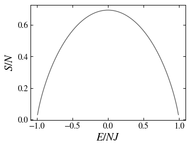
$$E = -\frac{\partial \ln Z }{\partial 1/T} = - NJ \tanh(J/T) = - NJ m$$

the entropy,

$$S = \frac{E-F}{T}= N \ln\left(2 \cosh\frac{J}{T}\right) - \frac{NJ}{T}\tanh\frac{J}{T}$$

which as a function of the energy shows a decreasing range, signaling the existence of negative temperatures EX (see the figure below).

For a two level system there exists a range of energies for which the entropy decreases, resulting, for high energies, in the appearance of negative temperatures.

It is interesting to show that the entropy as a function of the energy,

$$s = \frac{S}{N} = -\frac{1 + \epsilon}{2} \ln \frac{1 + \epsilon}{2} - \frac{1- \epsilon}{2} \ln \frac{1 - \epsilon}{2}\,, \epsilon = E/NJ$$

can also be obtained using the microcanonical ensemble EX.

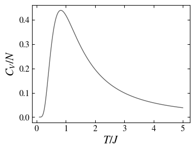
The heat capacity, or magnetic susceptibility $\chi = \partial M/\partial \mu_0 B \sim \partial N m/\partial J$, in the magnetic case ($J$ represents an applied magnetic field to the spin system), is the temperature derivative of the energy $E$,

$$C_V = \frac{NJ^2}{T^2} \cosh^{-2} \left(\frac{J}{T} \right) \rightarrow \frac{J^2}{T^2} \sim \frac{J^2}{T}\chi\,.$$

Note that the last expression is compatible with the Curie law $\chi \sim 1/T$ (at $J=0$).

The heat capacity of the paramagnet as a function of the temperature, showing a decreasing range at high temperature.

Comparing the two examples, the oscillators and the paramagnet, we observe that an essential difference is in the range of the allowed energies; while the system of oscillators allows arbitrary high energies, in the range $E/N \ge 1/2$, in the spin system the energy is restricted to a band $-1 \le E/N \le 1$; this is the physical origin of their fundamentally different thermodynamic behavior.

Ideal gas

To illustrate the use of the grand canonical ensemble we consider an ideal gas of mass $m$ particles in a volume $V$, in contact with a reservoir enabling the exchange of energy at temperature $T$ and molecules at chemical potential $\mu$. The $N$-particles hamiltonian is,

$$H_N(x, p) = \sum_{n=1}^N \frac{p_n^2}{2m}\,, \quad x \in V$$

where the only interaction is with the walls, imposing the restriction on the positions $x=\{ \boldsymbol x_1, \ldots, \boldsymbol x_N \}$. The canonical partition function for $N$ is

$$Z_N(T) = \frac{1}{N!}\int_\Gamma \prod_{n=1}^N \frac{\D \boldsymbol x_n \D \boldsymbol p_n}{(2\pi\hbar)^3} \exp\left( -\sum_{n=1}^N \frac{p^2_n}{2mT} \right)\,.$$

The integral over $x$ gives a factor $V^N$ and the integrals over the impulsions factorize in gaussian integrals for each particle, the result is EX,

$$Z_N(T) = \frac{V^N}{N!} \left( \frac{m T}{2\pi \hbar^2}\right)^{3N/2} = \frac{g^N}{N!}$$

where we defined the nondimensional parameter $g=g(V,T) = V/\lambda^3$, with $\lambda = (2\pi\hbar^2/mT)^{1/2}$. We are now ready to compute the grand partition function:

$$Z(T,\mu) = \sum_N \E^{\mu N/T} Z_N(T) = \E^{z g}\,,\quad z=\E^{\mu/T}\,,$$

from which we obtain the grand potential,

$$\Phi(T,\mu,V) = -T \E^{\mu/T} \frac{V}{\lambda(T)^3}$$

The thermodynamic quantities are obtained by derivation. The equilibrium number of particles is

$$N = -\frac{\partial \Phi}{\partial \mu} = \E^{\mu/T} \frac{V}{\lambda(T)^3}\,,$$

the pressure,

$$P = -\frac{\partial \Phi}{\partial V} = \E^{\mu/T} \frac{T}{\lambda(T)^3} = \frac{NT}{V}\,,$$

which coincides with the usual thermodynamic equation of state $PV=NT$. Note that the grand potential is $\Phi(T,\mu,V) = - P(T,\mu) V$. Putting $p_T = T/\lambda^3$, the chemical potential writes,

$$\mu = T\ln(P/p_T)$$

the Nernst equilibrium potential used in electrochemistry. The entropy is,

$$S = - \frac{\partial \Phi}{\partial T} = \frac{5N}{2} + N \ln \frac{V}{N\lambda^3}$$

and the internal energy,

$$E = \Phi + TS + \mu N = \frac{3N}{2}T$$

the equipartition result.

Rotation and vibration of a polyatomic gas

The molecules forming a gas, in addition to their translation degrees of freedom, are endowed with other dynamical internal degrees of freedom, such as vibrations or rotations. For instance, the atoms of a diatomic molecule can oscillate around their minimum energy configuration, or rotate around its center of mass. We will consider a diatomic molecule of distinguishable atoms, allowing us to use the Boltzmann distribution function (for identical atoms one should take into account spin effects). The vibrational energy is,

$$\epsilon_n = \hbar \omega \left(n+\frac{1}{2}\right)\,,$$

similar to the energy of a harmonic oscillator, where $\omega$ is the vibration frequency and $n=0,1,\ldots$ is the energy level quantum number. The rotation energy of an axisymmetric molecule depends on its inertia momentum $I$ and is proportional to the square of the angular momentum $L^2$,

$$\epsilon_l = \frac{\hbar^2 l(l+1)}{2I}\,,$$

where $l=0,1,\ldots$ is the orbital quantum number; each level is $2l+1$ times degenerate.

In the canonical ensemble, the part of the partition function associated with the vibration and rotation degrees of freedom of $N$ independent molecules, is given by the product of one particle partition functions, then

$$ Z = Z_I Z_r^N Z_v^N\,,\quad Z_r = \sum_l (2l+1) \E^{-\epsilon_l/T},\; Z_v = \sum_n \E^{-\epsilon_n/T} $$

gives the total partition function whith $Z_I$ and $Z_1$ the ideal gas (which takes into account the kinetic energy) and the one particle vibration and rotation contributions, respectively, and where the corresponding energy levels $\epsilon_s$ are counted with their degeneracy $g_s$.

Typical kinetic, rotation and vibration energies of the diatomic gas are,

$$T,\; \frac{\hbar^2}{I},\; \hbar \omega\,,$$

respectively. Their relative values give an order of magnitude of their contribution to the thermodynamic properties; for example, one may predict (actually, a quantum mechanical effect) that the rotation degrees of freedom are negligible when the parameter $\hbar^2/IT \ll 1$ is small, and similarly for the vibration when $\hbar \omega/T \ll 1$. This statement is in conflict with the equipartition theorem, which assign to each degree of freedom the same energy (note that the previous estimates include the quantum energy scale).

The partition function of the vibrational degrees of freedom is readily calculated:

$$Z_v = \sum_n \E^{-\Theta_v (n + \tfrac{1}{2})} = \frac{1}{2\sinh(\Theta_v/2)}\,,\quad \Theta_v = \frac{\hbar \omega}{T}\,.$$

The internal energy and heat capacity (at constant volume) are then,

$$E_v = N T^2 \frac{\partial \ln Z_v}{\partial T} = \frac{N\hbar\omega}{2} \coth \frac{\Theta_v}{2} \,,$$

and

$$C_v = \frac{N \Theta_v^2}{4} \sinh^{-2}\frac{\Theta_v}{2} \,,$$

respectively. In the high temperature limit $\Theta_v \ll 1$, one recovers the classical result of constant heat capacity $C_V \approx N$, while in the low temperature limit $\Theta_v \gg 1$, it vanishes exponentially

$$C_v \approx \frac{N \hbar^2 \omega^2}{4T^2} \exp(-\hbar\omega/T)\,, \quad T \ll \hbar\omega \,.$$

Vibrational heat capacity as a function of the temperature.

The one molecule partition function of the rotation degrees of freedom is given by,

$$Z_r = \sum_{l=0}^\infty (2l + 1) \E^{-\Theta_r l(l+1)}\,, \quad \Theta_r = \frac{\hbar^2}{2IT}\,,$$

where we defined the nondimensional parameter $\Theta_r$ that separates the quantum low temperature regime $\Theta_r \gg 1$ to the classical one, $\Theta_r \ll 1$. At low temperatures the exponential factors decrease rapidly, therefore, we can approximate the partition function by the first few terms,

$$ Z_r \approx 1 + 3 \E^{-2\Theta_r} + 5 \E^{-6\Theta_r}\,,\quad \Theta_r \gg 1\,. $$

At high temperatures, terms with angular momentum up to $l^2 \sim 1/\Theta_r$ will contribute to the sum; hence, we can use the approximation of the sum by an integral (Euler-MacLaurin):¹

$$Z_r \approx \frac{1}{\Theta_r} + \frac{1}{3} + \frac{\Theta_r}{15}\,,\quad \Theta_r \ll 1\,.$$

The first term,

$$\int_0^\infty \D l \, (2l+1) \E^{-\Theta_r l(l+1)} = \frac{1}{\Theta_r}$$

gives the classical value. Using these approximations, we can compute the thermodynamic quantities in the limits of low and high temperature:

$$\ln Z_r = \begin{cases} 3 \E^{-2\Theta_r} & \text{for } \Theta_r \gg 1\\ -\ln \Theta_r + \frac{\Theta_r}{3} + \frac{\Theta_r^2}{90} & \text{for } \Theta_r \ll 1 \end{cases} \,.$$

The energy is,

$$E_r = \begin{cases} \frac{3\hbar^2}{I} \E^{-2\Theta_r} & \text{for } \Theta_r \gg 1 \\ T - \frac{\hbar^2}{2I}\left( \frac{1}{3} + \frac{\Theta_r}{45}\right) & \text{for } \Theta_r \ll 1 \end{cases}$$

and the heat capacity,

$$C_r = \begin{cases} 12 \Theta_r^2 \E^{-2\Theta_r} & \text{for } \Theta_r \gg 1 \\ N + \frac{N}{45} \left( \frac{\Theta_r}{T}\right)^2 & \text{for } \Theta_r \ll 1 \end{cases} $$

Exact heat capacity at constant volume $C_r = (\Delta E_r/T)^2$, showing the exponential convergence to zero at low temperatures (quantum regime), and the asymptotic (classical) value of $N$ at high temperatures.

Sympy code for the high temperature expansion

%matplotlib inline
import matplotlib.pyplot as plt
import numpy as np
from sympy import *
init_printing()

It is convenient to choose units such that $\hbar = I = 1$, the unit of energy is then $\hbar^2/I$; the non dimensional parameter $\Theta_r$, becomes $\Theta_r = \hbar^2/2IT = 1/2T$.

l = Symbol("l", real = True)
T = Symbol("T", positive = True)
x = symbols("x")

Z = (2*l+1)*exp(-l*(l+1)/(2*T))
Z

$$\left(2 l + 1\right) e^{- \frac{l \left(l + 1\right)}{2 T}}$$

z = expand(integrate(Z,(l,0,oo)))
z

$$2 T$$

z0 = Z.subs(l, 0)
z0

$$1$$

z1 = diff(Z, l, 1).subs(l, 0)
z1

$$2 - \frac{1}{2 T}$$

z3 = expand(diff(Z, l, 3).subs(l, 0))
z3

$$- \frac{6}{T} + \frac{3}{T^{2}} - \frac{1}{8 T^{3}}$$

Euler-MacLaurin formula wiki

If $f$ is a sufficiently regular function decreasing at infinity ($\forall k$, $f^{(k)}(\infty) = 0$), the series,

$$S = \sum_{n = 0}^\infty f(n)$$

can be approximated by an integral,

$$S = \int_0^\infty \mathrm{d}n\, f(n) + \frac{f(0)}{2} - \sum_{k=1}^{K-1} \frac{B_{2k}}{(2k)!} f^{(2k-1)}(0) + R_K$$

where the $B_n$ are the Bernoulli numbers wiki,

$$B_2 = 1/6,\; B_4 = -1/30,\; B_6 = 1/42,\ldots$$

Zhigh = expand(z + z0/2 - z1/(6*2) + z3/(30*2*3*4))
Zhigh

$$2 T + \frac{1}{3} + \frac{1}{30 T} + \frac{1}{240 T^{2}} - \frac{1}{5760 T^{3}}$$

lnZ = series(log(Zhigh.subs(T, 1/x)), x, n = 3).subs(x, 1/T)
lnZ

$$\frac{1}{360 T^{2}} + \frac{1}{6 T} + \ln{\left (2 \right )} - \ln{\left (\frac{1}{T} \right )} + \mathcal{O}\left(\frac{1}{T^{3}}; T\rightarrow \infty\right)$$

This last expression gives the logarithm partition function expansion for large temperatures:

$$\ln Z_r \approx \ln(2T) + \frac{1}{6T} + \frac{1}{360T^2}$$

exact to $1/T^2$ terms.

Er = expand(T**2 * diff(lnZ, T))
Er

$$- \frac{1}{180 T} - \frac{1}{6} + T + \mathcal{O}\left(\frac{1}{T^{2}}; T\rightarrow \infty\right)$$

cr = expand(diff(Er,T))
cr

$$\frac{1}{180 T^{2}} + 1 + \mathcal{O}\left(\frac{1}{T^{3}}; T\rightarrow \infty\right)$$

The figure below represents schematically the behavior of the heat capacity as a function of the temperature.

Schematic total $C_V$ of a diatomic molecule, showing the transtaltion, rotation and vibration contributions, appearing at different temperatures.

We note that the classical prediction $c_V = 7/2$ is reached at very high temperatures, when the rotational and vibrational degrees of freedom are excited. For example the O$_2$ molecule has a rotation temperature of about $2\,$K, and a vibration temperature of $2200\,$K; therefore, at normal temperature the measured heat capacity is $5/2$.

We used the Boltzmann distribution to compute the partition function and the corresponding thermodynamics; it cannot account to the behavior of the system at very low temperatures. For instance, the heat capacity must vanish at $T=0$. To obtain the correct low temperature behavior one needs quantum statistics (for bosons or fermions). We also neglected the possibility of phase transitions: at low temperatures liquid and solid states naturally appear.

Notes

Euler-McLaurin formula
$$ \sum_{n=0}^\infty f(x) = \int_0^\infty \D x f(n) + \frac{f(0)}{2} - \frac{f'(0)}{12} + \frac{f'''(0)}{720} + \cdots $$
↩