Problems and exercises | Random physics

$\newcommand{\I}{\mathrm{i}} \newcommand{\E}{\mathrm{e}} \newcommand{\D}{\mathop{}\!\mathrm{d}} \newcommand{\bra}[1]{\langle{#1}|} \newcommand{\ket}[1]{|{#1}\rangle} \newcommand{\braket}[1]{\langle{#1}\rangle} \newcommand{\bbraket}[1]{\langle\!\langle{#1}\rangle\!\rangle} \newcommand{\bm}{\boldsymbol}$

Lectures on statistical mechanics.

Selected problems

1

Microcanonical ensemble: the harmonic oscillator. Compute the volume of phase space inside the surface of constant energy $H < E$ ($H$ is the hamiltonian of a system of $N$ oscillators). Deduce the entropy. Show that the result do not depend on the value $\Delta$ of the energy shell thickness.

Solve the same problem for a set of $N$ quantum harmonic oscillators, taking into account that bosons are indistinguishable.

Compare the expression of the energy as a function of the temperature in both, classical and quantum, cases.

2

Canonical and grand canonical ensembles: classical disordered system. Calculate the canonical partition function of a system whose hamiltonian energy is

$$ H = \sum_n \frac{p_n^2}{2m} + \sum_n \sum_x V(\bm r_n - R_x) $$

where $n$ labels the particle ($n=1,\ldots,N$, for $N$ particles) and $x$ labels the impurities located at random positions $\bm R_x$ ($x = 1, \ldots, N_i$, for $N_i$ impurities); $p_n$ and $r_n$ are the momenta and positions of the particles. Using the canonical partition function for $N$ particles $Z_N(T,V)$, compute the grand canonical partition function $Z(\mu,T,V)$ ($T$ is the temperature, $\mu$ the chemical potential, and $V$ the volume).

Assume that the potential energy of an impurity is attractive $-V_0$ (in the region $R<a$), and that their distribution is uniform in the system’s volume $V$ (of density $n_i = N_i/V$ small enough to avoid overlaps). Using these assumptions calculate the averaged value of the logarithm of $Z$ and show that

$$ \braket{\ln Z(\mu,T,V)} = \frac{\E^{\mu/T} V}{\lambda^3} \E^{n_i f}, \quad f = \int \D \bm R (\E^{-V(\bm R)/T} - 1) $$

From the expression of the thermodynamic potential obtain the equation of state. Compare it to the one of an ideal gas.

3

Random matrices. Find the Wigner surmise

$$ p(s) = \frac{\pi s}{2} \E^{-s^2/4} $$

for the level spacing distribution of orthogonal random matrices, using the case of a $2 \times 2$ matrix.

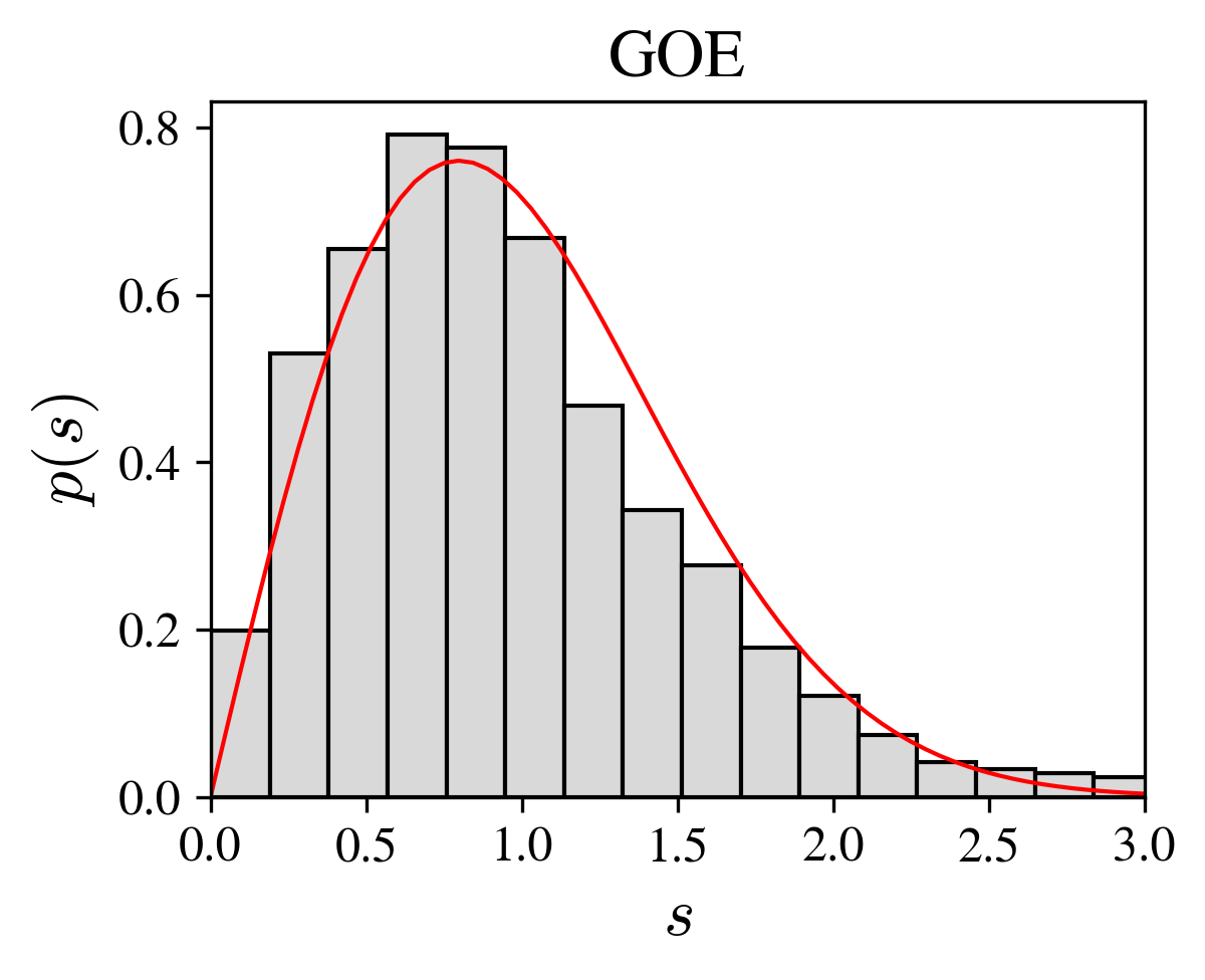
Wigner surmise (red line) and histogram of a single large matrix.

Investigate the properties of the spectrum numerically.

"""Compute the level spacings of a matrix in the GOE"""
import numpy as np
from scipy.linalg import eigvalsh
rng = np.random.default_rng(523) # seed
n = 1000 # matrix size
g = rng.normal(0, 1, (n,n)) # nxn gaussian numbers
h = (g + g.T)/2 # real symmetric
e = eigvalsh(h) # eigenvalues
e = np.sort(np.real(e))
s = np.diff(e)/np.mean(np.diff(e)) # level spacings

4

Identity of particles. Find the joint probability density of 2 bosons (and 2 fermions) to be at positions $\bm x_1$ and $\bm x_2$,

$$ \braket{\bm x_1 \bm x_2 | \rho(H) | \bm x_1 \bm x_2} $$

using the canonical quantum ensemble

$$ \rho(H) = \frac{\E^{-H/T}}{Z_2(T,V)}, \quad H = \frac{\bm p_1^2 + \bm p_2^2}{2m} $$

density matrix; $H$ is the hamiltonian of the two identical particles.

Show that it is given by the formula

$$ \braket{\bm x_1 \bm x_2 | \rho(H) | \bm x_1 \bm x_2} = \frac{1}{2\lambda^6 Z_2} \big(1 \pm \E^{-2\pi |\bm x_1 - \bm x_2|^2/\lambda^2}\big) $$

where $\lambda$ is the thermal length at temperature $T$. Deduce the expression of the two particles partition function $Z_2(T,V)$, and compare the result with the classical one.

5

Bose-Einsein condensate. Demonstrate that $N$ free bosons in two dimension do not form a condensate; show in particular that the critical temperature $T_c$ (signaling the quantum dominated regime) vanishes like $T_c \rightarrow 1/\ln N$ in the thermodynamic limit.

In contrast to the free case, demonstrate that in a harmonic trap, a two-dimensional gas of bosons do forms a condensate. Show that in this case the critical temperature is

$$ T_c = \frac{\sqrt{6}\hbar \omega}{\pi} N^{1/2}, $$

where $\omega$ the harmonic oscillator frequency.

6

Thermionic emission. Electrons in a metal at temperature $T$ can escape the surface energy barrier $-W$ if their velocity $p_z/m$ (perpendicular to the surface) satisfies $p_z > \sqrt{2 m W}$ ($m$ is the electron mass and $\bm p$ its momentum). Using the Fermi-Dirac distribution $n_\epsilon$ show that the thermionic current is

$$j = \frac{emT^2}{2\pi^2 \hbar^3} \exp\left(-\frac{W - \epsilon_F}{T}\right)$$

where $\epsilon_F$ is the fermi energy ($k_\mathrm{B} = 1$).

Use units such that $e = W = m = \hbar = 1$. Assume that typical particle energies are larger than $W$ (otherwise emission is impossible). Compare the quantum result with the classical one.

7

Paramagnetism and diamagnetism. The energy of a particle in a magnetic field $\bm B$ is, firstly neglecting the orbital contribution,

$$ H = \frac{p^2}{2m} + \mu_B \bm \sigma \cdot \bm B, \quad \epsilon_{\bm k} = \frac{(\hbar k)^2}{2m} \pm \mu_B B, $$

where $\bm \sigma \cdot \bm B$ has eigenvalues $\pm 1$ ($m$ is the particle mass, $\hbar \bm k$ its momentum $\bm p$ eigenvalue, and $\mu_B$ the Bohr magneton; we put $g=2$). Find the magnetic susceptibility $\chi = \mu_0 M/B$ (at zero field, $\mu_0$ is the vacuum permeability).

Secondly, compute the orbital contribution to the susceptibility, coming from the kinetic term:

$$ H = \frac{(\bm p + e\bm A)^2}{2m}. $$

Investigate the high and low temperature limits.

8

Mean field. The hamiltonian of an ising model in a regular lattice of $N$ sites with $q$ neighbors is

$$ H = -J\sum_{\braket{x,y}} s_x s_y $$

where $s_x = \pm 1$ is the spin on site $x$; $y \in N(x)$ is a neighbor of $x$ belonging to the set $N(x)$ of size $q$; $J$ is the exchange parameter. In the Bethe approximation, which is a generalization of the standard mean-field model, one considers a given spin $s_0$ and its neighbors:

$$ H(s_0) = -Js_0 \sum_{y \in N(0)}s_y - h \sum_{y \in N(0)}s_y = H_c, $$

where the last term contains the information about the local field $h$ created at the site $0$ by the neighboring spins $y \in N(0)$. $H_c$ is the “cluster” hamiltonian, it depends on the unknown parameter $h$, which should be determined self-consistently to match the expectation value of the observables (like the magnetization $m = \braket{s_x}$).

Using the “cluster” partition function

$$ Z_c = \mathrm{tr} \, \E^{-H_c(h)/T} = \sum_{s_x = \pm 1} \E^{-H_c(h)/T}, $$

compute $\braket{s_0}$ and $s_x$. From the condition of homogeneity (at equilibrium) $m = \braket{s_0} = \braket{s_x}$ for all $x$, deduce the self-consistent condition

$$ \frac{\cosh^{q-1}[(J+h)/T]}{\cosh^{q-1}[(J-h)/T]} = \E^{2h/T} $$

which determines $T_c$:

$$ T_c \approx \frac{2J}{\ln\frac{q}{q-2}}. $$

Compare the result for $q=4$ (square lattice) with the Onsager exact value of $T_c$.

Show that near the ferromagnetic transition, the magnetization behaves as $m \sim |T-T_c|^{1/2}$:

$$ m^2 \approx \frac{3 q}{q-1} \frac{q}{2} \ln \left( \frac{q}{q-2} \right) \left( 1 - \frac{T}{T_c} \right). $$

Verify that this formula reduces to the standard one (mean field) in the limit $q \rightarrow \infty$.

9

Mean field and Landau theory. Helium ($^4\mathrm{He}$) liquefies at $T_l \approx 4\,\mathrm{K}$ (at normal pressure), and undergoes a phase transition around $T_c \approx 2.2\,\mathrm{K}$ towards a superfluid state, the so-called $\lambda$-transition. If the helium liquid contains a fraction $c_3$ of the $^3\mathrm{He}$ isotope, the nature of the superfluid transtion changes when $x > x_t = c_3/(c_3 + c_4) \approx 0.67$, the tricritical point ($c_4$ is the $^4\mathrm{He}$ concentration): it is second order for $x<x_t$, and first order when the mixture when $x > x_t$, which results in the separation into rich in helium-3 and rich in helium-4 phases. A simple model to describe the properties of the tricritical point $(x_t, T_t)$, was proposed by Blume, Emery and Griffiths (1971). It is based on the hamiltonian

$$ H = -J \sum_{\braket{i,j}} S_i S_j + \Delta \sum_i (S_i^2 - 1), \quad S_i = 0, \pm 1 $$

where $S_i = \pm 1$ represents the helium-4 interacting atoms and $S_i = 0$ the helium-3 atoms, treated as impurities, $\Delta$ controls the number of helium-3 atoms (it is proportional to the difference of chemical potentials); the sums extend to the total number of lattice sites $N$, and $\braket{i,j}$ labels neighbors. The concentration of $^3\mathrm{He}$ is then $x = 1 - \braket{S_i^2}$.

Show that the probability distribution P(S) is given by

$$ P(S) = \frac{\E^{(qJmS - \Delta S^2)/T}}{Z}, \quad Z = 1 + 2\E^{-\Delta/T} \cosh\big(qJm/T\big). $$

You may use the minimization of the free energy $F$, assuming that $S_i$ are independent random variables (mean field approximation):

$$ F = \braket{H} + NT\sum_S P(S) \ln P(S), $$

where we also exploit homogeneity. Compute the expected value of $S^2$:

$$ \braket{S^2} = \frac{2\E^{-\Delta/T} \cosh(qJM/T)}{Z}. $$

Deduce the free energy per atom $f(m; T, \Delta) = F/N$

$$ f = \frac{1}{2} qJm^2 - T \ln \left( 1 + 2 \E^{-\Delta/T}\cosh \frac{qJm}{T} \right) - \Delta. $$

Just above the transition (disordered state) $m = 0$; you can then expand $f(m)$ in powers of $m$ up to the 6th order. Analyse the possible phase transitions using Landau approach. Compute, in particular, the values of the concentration $x_t$ and the temperature $T_t$ at the tricritical point.

Numerical application: plot the phase diagram in the $(x,T)$ plane.

Probability¹

1

Characteristic functions. Calculate the characteristic functions, and the first moments (mean, variance) of the probability densities: uniform $\sim 1$, Laplace $\sim \E^{-|x|}$, Gaussian $\sim \E^{-x^2}$, Maxwell $\sim x^2 \E^{-x^2}$, Cauchy $\sim 1/(1+x^2)$, and Rayleigh, $\sim x \E^{-x^2}$. Note that only the behavior of the functions is given, you must find, adding the necessary parameters, their complete expression, satisfying the normalization.

2

Random walk. A particle moves in space by steps of length $a$ and orientation $(\theta,\varphi)$ (the azimutal and polar angles) with probability,

$$p(\theta, \varphi) = \frac{\sin\theta}{4\pi}\,,$$

(explain this formula).

Calculate the moments up to second order of the cartesian coordinates $\boldsymbol x =(x,y,z)$ after $N$ steps.
Use the central limit theorem to find $p(\boldsymbol x)$.

3

Typical maximum value. If $X = \{x_1,\ldots,x_n\}$ is a set of random independent variables, uniformly distributed in $[0,1]$, show that the variance around $x = \max X$ tends to zero with $n$. Find first the probability $p_n(x)$ in terms of the $p(x_i < x)$, where $i=1,2,\ldots$, and then calculate the mean and variance of $x$.

4

Information and entropy. Use the maximum entropy principle to find the distribution $p(v)$ of the velocity $v$ of one particle subject to the constraints: (V) $\braket{|v|} = c$, (E) $\braket{mv^2/2} = mc^2/2$. Show that the energy constraint (E) contains more information than the mean velocity constraint (V),

$$I_\text{E} - I_\text{V} > 0$$

compute this information difference in bits.

5

A simple model of a polymer consists in a chain of bonded atoms ($a$ is the link length) whose successive links can make an angle of $0$ or $\pi$, with probability $1/2$, for a total length $L$.

Find the number $\Omega$ of chains of length $L$ as a function of the number of atoms $N$. You may introduce the number of $0$ links $N_+$ and the number of $\pi$ links, such that $L=(N_+ - N_-)a$ and $N = N_+ + N_-$.
Assume $L/a \ll N$ and show that $\Omega(N,L)$ approaches a gaussian distribution of variance $\sim N$ (as in a random walk). Deduce the entropy (using the Stirling approximation).
Show that the force required to maintain the chain length at a fixed value $L$ follows the Hooke’s law (for a well folded chain).
If $L$ can take any value, not necessary small with respect to $Na$, use the Boltzmann weight $\sim \E^{-V/T}$ ($V$ is the potential of the external force), to demonstrate that the force is,

$$f = \frac{T}{a} \mathrm{artanh}\left( \frac{L}{Na} \right)\,.$$

(Hint. Consider one link.)

6

We consider first, a random symmetric $N \times N$ matrix $M$, each element $i \le j$ distributed according to

$$p(x) = p(M_{ij}=x) = \begin{cases}\frac{1}{2a} & \text{for} \quad x\in (-a,a)\\ 0 & \text{otherwise}\end{cases}\,.$$

Calculate the characteristic function $p(k)$ of the distribution $p(M)$ and of the distribution of the trace $\mathrm{Tr}\,M$, $p_T(k)$.
For large $N$ the cumulant of $N$ elements is $N$ times the cumulant of one element. Use the central limit theorem (gaussian distribution for large $N$) to compute $p(t)$, with $t = N^{-1/2} \mathrm{Tr}\, M$; show that,
$$p(t) = (3/2\pi a^2)^{1/2} \E^{-3t^2/2a^2}\,.$$

Consider now that $M$ is a $2\times2$ gaussian random matrix: each element is normally distributed with $\mathcal{N}(0,1)$ for the diagonal elements, and $\mathcal{N}(0,1/\sqrt{2})$ for the nondiagonal ones. (We denote $\mathcal{N}(0,\sigma)$ a normal distribution with zero mean and variance $\sigma^2$.)

Compute the eigenvalues $\lambda_\pm$ of $M$ and show that the probability distribution of the “spacing” $s = (\lambda_+ - \lambda_-)/\Delta$, where $\Delta$ is such that the mean spacing is unity, is given by the Wigner surmise:
$$p(s) = \frac{\pi s}{2} \E^{-\pi s^2/4}\,,$$
where the mean value and normalization satisfy,
$$\int_0^\infty \D s\, p(s) s = \int_0^\infty \D s\, p(s) = 1\,.$$
Verify numerically that the Wigner surmise correctly fits the level spacing histogram of large random symmetric matrices.

Noninteracting systems: Boltzmann²

1

A system, satisfying Boltzmann statistics, consists in $N$ two level atoms (with energies $E_1 < E_2$); the system is in contact with a reservoir at temperature $T$. If the emission of a quanta into the reservoir occurs, the level populations change $n_2 \rightarrow n_2 - 1$ and $n_1 \rightarrow n_1 + 1$. Assuming $n_1 \gg n_2$, calculate the entropy change for the two level system and the reservoir; eventually derive the Boltzmann relation for the ration $n_2/n_1$.

2

Show that an ideal gas, in the diluted, high temperature limit $n \lambda^3 \ll 1$, the fermi distribution reduces to the boltzmann one ($n$ is the density, $\lambda^2=2\pi \hbar^2/mT$, with $m$ the atom’s mass, and $T$ the temperature). Using the free particles density of states in a volume $V$, demonstrate that the ideal gas chemical potential $\mu$ is given by

$$\E^{\mu/T} = n\lambda^3.$$

3

Disordered material. An alloy contains a small fraction of impurities that can be in two energy states $\Delta_x > 0$ or $-\Delta_x$, according to their position $x$ in the crystal lattice. We assume that the impurities are independent. We are interested in the low temperature limit $T \ll \Delta$.

In the case that each impurity atom has the same levels $\pm\Delta$ (independent of position), calculate their contribution to the heat capacity (neglect all other possible contributions).
In the inhomogeneous case, write the total heat capacity summing up the individual contributions. Assuming now that the distribution of energy levels is exponential,
$$\rho(\Delta) = \frac{\E^{-\Delta/\Delta_0}}{\Delta_0}\,,$$
replace the sum by an integral, and investigate the low temperature behavior of the heat capacity. Compare with the homogeneous case.

4

Three level molecule. The lowest energy levels of a molecule are $E=0,\epsilon,10\epsilon$.

Compute the level population assuming boltzmann statistics (give the validity condition for this assumption), and compare the results. Find the temperature $T_c$ below which the highest level is empty.
Calculate the (exact) energy $E$ and specific heat $C_V$. Investigate the high and low temperature limits. Sketch $C_V=C_V(T)$.

5

The effective interaction energy between the two hydrogen atoms of a $\mathrm{H}_2$ molecule is

$$V = \epsilon \big[\E^{-2\kappa(r -r_0)} - 2 \E^{-\kappa(r - r_0)} \big]\,,$$

with the parameters: hydrogen mass $m = 1.672\, 10^{-27}\,\mathrm{kg}$, $\epsilon = 7\,10^{-19}\,\mathrm{J}$, $\kappa = 2\,10^{10} \, \mathrm{m^{-1}}$, and $r_0= 8\,10^{-11}\,\mathrm{m}$

Estimate $T_\text{R}$ and $T_\text{V}$, the threshold temperatures at which rotation and vibration degrees of freedom contribute to the specific heat $C_V$ of the diatomic gas.
Approximately calculate the values of the volume $C_V$ and pressure $C_P$ specific heats at $T[\mathrm{K}] = 25, 250, 2500, 10\,000$.

(Hint. Order of magnitude calculation, compute the relevant parameters from the potential shape and use dimensional like analysis.)

6

A high temperature hydrogen plasma contains a fraction ($T < m_\mathrm{e}c^2$) of positrons created through electron collisions $\mathrm{e}^{-} + \mathrm{e}^{-} \rightarrow 2\mathrm{e}^{-} + (\mathrm{e}^{+} + \mathrm{e}^{-})$, or proton-electron collisions $\mathrm{e}^{-} + \mathrm{p} \rightarrow \mathrm{e}^{-} + \mathrm{p} + ( \mathrm{e}^{+} + \mathrm{e}^{-})$ (note that the total charge is conserved). The proton density is $n_\mathrm{p} = 1\,10^{16}\,\mathrm{m^{-3}}$. Find the chemical potential for $\mathrm{e}^{-}$ and $\mathrm{e}^{+}$ and estimate the temperature at which the positron density is $n_+ = 1\,10^{6}\,\mathrm{m^{-3}} \ll n_\mathrm{p}$ and $n_+ = 1\,10^{16}\,\mathrm{m^{-3}} \approx n_\mathrm{p}$. Assume the plasma non relativistic and non degenerated.

7

An ideal gas of polar polar molecules is placed in a uniform electric field $\mathcal{E}$. The dipolar moment of each molecule is $p$, whose energy is $-p\mathcal{E} \cos \theta$, where $\theta$ is the angle between the applied field and the dipole. Compute the classical partition function $Z$ in the canonical ensemble, the mean polarization and the dipolar susceptibility $\chi = \D \braket{p}/ \D \mathcal{E}$, and the specific heat at constant volume. Find the high temperature asymptotics, where the classical approximation is valid.

8

Surfactant gas. A surfactant is diluted in an aqueous solution; the molecules binding energy in volume is $\epsilon$ and on the surface is $\epsilon_s$, the difference $\Delta \epsilon = \epsilon - \epsilon_s >0$. Suppose the surfactant molecules as an ideal gas of dimension $D$ and compute the partition function $Z(T,\mu_D,V_D)$ in the grand canonical ensemble; calculate the number $N_3$ of molecules in the volume $V_3 =V$ and $N_2$ of molecules on the surface $V_2 = A$. Find the ratio $N_2/N_3$ and discuss your result.

9

Relativistic gas. A one dimensional system of $N$ identical particles move in one dimension. The system’s classical hamiltonian is,

$$H= \sum_n [c |p_n| + w(x_n)]$$

where the potential energy vanishes in the region $0 \le x_n \le L$ and is infinite at the $x=0,L$ walls. Consider the microcanonical ensemble and calculate the number of states in phase space $\Omega(E,L,N)$ in the limit of large $N$. Observe that each momentum can have two signs and that $E=\sum_n |p_n|$ is conserved. Calculate the entropy, the equation of state and the heat capacities at constant length and constant pressure.

(Hint. The volume of a pyramide $\sum_n^N x_n \le L$, in $N$ dimensions is $L^N/N!$)

10

A gas of $N$ hard spheres of volume $v$ occupies a volume $V$. Compute the $\Omega(T,V,N)$ (microcanonical ensemble),

$$\Omega = \frac{1}{N!(2\pi \hbar)^N}\int_{H=E} \prod_{N=1}^N \D p_n \D x_n$$

with $E = \sum_n p_n^2/2m$. For the configuration integral assume that one can introduce successively one sphere into the system. Discuss the validity of this approach. Deduce the entropy of the gas, the equation of state and the isothermal compressibility $k_T$. (Read the interesting paper by Ursell 1927.)

Noninteracting systems: Bose and Fermi

1

Investigate how the usual laws of Stefan black body radiation $\sim T^4$, and Debye specific heat of a solid $\sim T^3$, are modified if one assumes that the spatial dimension is $D$.

2

Graphite is a stack of weakly coupled flat crystal layers of carbon atoms; experiments show that, instead of the usual Debye scaling with the temperature, the specific heat of graphite is proportional to $T^2$. Explain this behavior. You may assume that oscillations are two dimensional and the sound velocity is anisotropic (one mode through the layers, and two modes, on the layer plane).

3

Identical particles. A system consists in two identical non interacting particles in contact with a bath at $T$. Calculate the partition function of the two particle system $Z_2$ in terms of the one particle $Z_1$, in the case of bosons and fermions (spinless). Assuming that $Z_1 = V/\lambda^3$, compute the thermodynamics of the two particles system: energy, pressure and heat capacity at constant volume.

4

Bose gas in $D$ dimensions. Generalize the computation of a free Bose gas $\epsilon = p^2/2m$, to $D$ dimensions. Calculate the grand potential $\Phi_D(T,\mu,V)$ by approximating the sum over energies by an integral. Establish the range of validity of this approximation and, if necessary, separate the fundamental state from the integral in the computation of the number of particles. Deduce the thermodynamic properties, $N$, $P$, $E$ and $C_V$. Sketch $C_V(T)$ for all temperatures.

5

A fermion gas is confined in a two dimensional device. Compute the fermi energy, and the chemical potential as a function of the temperature.

6

White dwarf. Compute, using relevant physical approximations, the gravitational equilibrium of a sphere of degenerate electrons in the non-relativistic case. Establish the mass-radius relation. Discuss the orders of magnitude and the validity of the approximations. Show that in the limit of ultra-relativistic electrons there is a mass limit for stability.

Interacting systems³

Virial expansion

1

The interactions of argon atoms in a classical gas is roughly approximated by the potential,

$$w(r) = \begin{cases} \infty & \text{if } r < a \\ -\epsilon & \text{if } x \in (a,b) \\ 0 & \text{if } x > b \end{cases}\,,$$

where $r$ is the interparticle distance, $a$ is the repulsion radius, and $b$ the range of the attractive energy, of the order of $\epsilon$. Compute the second virial coefficient $B_2(T)$,

$$B_2(T) = 2\pi \int_0^\infty r^2 \D r\, \left(1 - \E^{-w(r)/T} \right)\,,$$

and discuss its behavior as a function of the temperature $T$.

Using the experimental values of the Boyle temperature $T_B = 410\,\mathrm{K}$, and the Joule-Thomson inversion temperature $T_i=720\,\mathrm{K}$, find approximate values of the interaction parameters $\epsilon$ and $a/b$. At the Boyle temperature $B_2=0$, the virial coefficient vanishes (ideal gas behavior due to the balance between attractive and repulsive molecular forces). At the inversion temperature the thermal expansion coefficient satisfies,

$$\alpha = \frac{1}{V} \left(\frac{\partial V}{\partial T} \right)_P = \frac{1}{T} \,,\quad T = T_i\,,$$

which is true for an ideal gas; this condition is equivalent to:

$$\frac{\D B_2(T)}{\D T} = \frac{B_2(T)}{T}\,,$$

defining the Joule-Thomson temperature. Above this inversion temperature, a free expanding gas raises its temperature, in contrast to the usual freezing effect.

2

Compute the second virial coefficient far a classical gas whose interaction is the purely repulsion potential,

$$w(r) = \frac{A}{r^\alpha}, \quad \alpha > 3\,.$$

Derive the expressions for the free energy, the entropy and the internal energy; calculate the equation of state.

Hint:

$$F = F_I + NT\sum_{k \ge 2} B_k(T) \frac{n^{k-1}}{k-1} \approx F_I + T B_2(T) \frac{N^2}{V}$$

where $F_I = NT \ln(n/\E \lambda^3)$ ($\lambda$ is the thermal length), with $n=N/V$, is the ideal gas free energy.

Lattice systems

3

The hamiltonian of the Potts model, a generalization of the ising model for $q$-states atoms, is written,

$$H = -J \sum_{x=1}^N \delta(s_x,s_{x+1}),\quad s_x = 1,\ldots,q$$

where $\delta$ is the kronecker symbol, for a one-dimensional system with periodic boundary conditions (and the number of lattice sites is macroscopic, $N \rightarrow \infty$).

Find the partition function using the transfer matrix method. Find the free energy for arbitrary $q$, starting with the special (ising) case $q=2$. Compute the energy and discuss the low and high temperature limits. Using the definition of the correlation length in terms of the first two largest eigenvalues $\lambda_1 > \lambda_2$, of the transfer matrix:

$$\xi^{-1} = \ln(\lambda_1/\lambda_2)$$

Analyse the behavior of $\xi = \xi(T)$, and show that there is no phase transition at finite temperature.

4

We want to investigate the behavior of the per site magnetization $m$ of a ferromagnetic material, using a simple phenomenological model. In the mean field approximation one neglects the fluctuations around the thermodynamic mean value. Find the effective hamiltonian of an ising model in a $D$-dimensional lattice,

$$H =-J \sum_{\braket{x,y}} s_x s_y - B \sum_x s_x, \quad s_x = \{-1,1\}\,,$$

in this approximation (the summation is over nearest neighbors). Show the existence of a phase transition between a low temperature ferromagnetic state and a high temperature paramagnetic state.

Compute the characteristic exponents, around the phase transition,

of the magnetization as a function of the temperature for vanishing field, and also as a function of the field for $T=T_c$ (the critical temperature); and
of the susceptibility.

Hint: exponent definitions,

$m(T) \sim |t|^\beta$, for $B=0$,
$B(m) \sim m^\delta$, for $T=T_c$,
$\chi \sim t^{-\gamma}$ for $T>T_c$ and a similar equation for $T<T_c$,

where $t = (T-T_c)/T_c$. Show that the free energy, near the transition can be expanded in powers of the magnetization $m$.

5

Duality relation in the twodimensional ising model. Compute the partition function using series expansions at low and high temperatures. We denote $K=J/T$ the effective coupling and $N$ the number of spins in the square lattice.

Show that at low temperature the successive terms of the expansion correspond to flipping one spin, two neighbor spins, two isolated spins, etc.:

$$Z_{L} = 2 \E^{2NK} \left(1 + N u^4 + 2N u^6 + \cdots \right), \quad u = \E^{-2K}$$

Show that at high temperature the expansion depends on the perimeter (number of bonds) of closed path in the lattice, leading to an expansion on the closed graphs (single unit square, two neighboring unit squares, etc.):

$$Z_{H} = 2^N \cosh^{2N}K \left(1 + N t^4 + 2N t^6 + \cdots \right), \quad t = \tanh K$$

Compare the two series and deduce that there must be a relation between the high and low constants ($K_L = K$ and $K_H = K^\star$, $\tanh K = \E^{-2K^\star}$) leading to the duality relation:

$$\frac{Z(K)}{\sinh^N (2K)} = \frac{Z(K^\star)}{\sinh^N (2K^\star)}$$

where we used that $\sinh (2K) \sinh (2K^\star) = 1$ (exercice).

Phase transitions

6

Stoner model of magnetism. In an electron gas the fermi statistics repulsion (antisymmetric wave function) favors spin alignement (symmetric wave function). A simple expression of the spin-dependent repulsion energy is,

$$w = \frac{\alpha}{V} N_+ N_-, \quad N=N_+ + N_-\,,$$

where $\alpha$ is a phenomenological energy parameter and $N$ the total number of particles, sum of spin up $N_+$ and spin down $N_-$ electron numbers (the volume factor ensures that $U$ is extensive).

Calculate the fermi energy of the spin up and down electrons (assume low temperature $T$). Deduce the expression of the total kinetic energy as a function of the up and down densities.
Assume that the density difference $\Delta n$ with respect to the non magnetic state $N_+=N_-=N/2$, $n_\pm = n/2 \pm \Delta n/2$, is small $\Delta=\Delta n/n \ll 1$. Compute the total energy as an expansion to fourth order in $\Delta n$.
Show that the paramagnetic state is unstable for some $\alpha > \alpha_c$, compute the critical interaction $\alpha_c$, indicating the presence of a quantum phase transition. Investigate the behavior of the magnetization around the transition as a function of $\alpha$, $M = M(\alpha)$.

7

The Landau free energy of a ferromagnetic system is;

$$ F[\phi,H]=\int_{\mathrm{Vol}} \mathrm{d}x \left[ \frac{\kappa}{2}(\nabla \phi)^2 + V(\phi) - \phi H\right], $$

where the order parameter $\phi=\phi(x)$ is related to the magnetization density (in one direction); the thermodynamic potential is a pair function of the order parameter, in order to satisfy the system’s invariance with respect to the inversion of the external field (even in the zero field limit),

$$ V(\phi) = a \phi^2 + b\phi^4, $$

$\kappa,a,b$ are phenomenological constants, in principle dependent on the temperature, and the last term is the coupling with an external magnetic field $H$ (in energy units).

Find the minimum of $F$ from the first variation $\delta F/\delta \phi=0$,

$$ -\kappa \nabla^2 \phi + 2 a \phi + 4 b \phi^3 =0\; \Rightarrow\; \phi=m=\left\{0, \pm \sqrt{-a/2b}\right\}, $$

where $m=m(T)$ is the equilibrium magnetization (per unit volume). Show that the phase transition occurs at $a(T=T_c)=0$; for $a>0$ the only stable minimum corresponds to $\phi=0$; for $a<0$ two opposite values of the magnetization arise. Assuming that $a$ is a smooth function of the temperature, $a=a_0(T-T_c)$ to lowest order, near the critical temperature, compute the magnetization,

$$ \phi\sim|T-T_c|^{\beta} $$

and find the exponent ($\beta=1/2$ corresponding to the mean field prediction.

The validity of this result is limited by the existence of large spatial fluctuations intrinsic to the phase transition. In order to study these fluctuations compute the second variation of the free energy:

\begin{align*} m(x) &= -\frac{\delta F}{\delta H(x)},\\ \chi(|x-x'|) &= \frac{\delta m(x)}{\delta H(x')} = -\frac{\delta^2 F}{\delta H(x) \delta H(x')}, \end{align*}

where $\chi=\chi(T)$ is the susceptibility; it characterizes the linear response of the magnet to a small applied magnetic field. In a translation invariant system it depends on the distance between two points $x$ and $x'$. Using the fluctuation-dissipation theorem, $\chi=TG$ ($k_\mathrm{B}=1$), show that the equation for the correlation function $G$, writes,

$$ \left[-\nabla^2 + \xi(T)^{-2}\right] G(x-x') = \frac{T}{\kappa}\delta(x-x'), $$

with the correlation length $\xi$. Demonstrate that $\xi = [\kappa/2a_0(T-T_c)]^{1/2}$, in the paramagnetic state, and $\xi = [-\kappa/4a_0(T-T_c)]^{1/2}$, in the ferromagnetic state.

This length characterizes the exponential decay of correlations outside the transition. The correlation length diverges at the transition temperature, $\xi\rightarrow\infty$ for $T\rightarrow T_c$.

Finally, show that at the transition, the correlation function decays algebraically in dimension $d>2$

$$ G(x) \sim \frac{1}{x^{d-2}}, $$

which is a consequence of the divergence of the correlation length below $T_c$.

Glauber dynamics

8

A general Ising system of spins is defined by the hamiltonian

$$H = -J\sum_{\langle x, y\rangle} s_x s_y$$

where the sum runs on the lattice neighbors. At time $t$ a random spin $x$ is selected and its state changed with a probability $w_x$ that depends on the local magnetization (the sum of the spins of its neighbors):

$$w_x[s]= \frac{1}{2} \left[ 1- s_x \tanh \left( \beta \sum_{y\in \langle x \rangle} J s_y \right) \right].$$

is the transition rate form configuration $s$ to configuration $s'=s^{(x)}$ with $s_x \rightarrow - s_x$ flipped. Glauber dynamics can be viewed as a stochastic equation that, at each time step $\Delta t$, updates the spins according to the rule:

$$s_x(t+\Delta t) = \begin{cases} s_x & \text{with prob } 1 - \Delta t\, w_x \\ -s_x & \text{with prob } \Delta t\, w_x \end{cases}$$

from which one can deduce the evolution equations for the spin moments $S_x =\langle s_x \rangle$, $S_{xy} = \langle s_x s_y \rangle$, etc.

In the mean field approximation one neglects local spin fluctuations $s_x\approx \langle s_x\rangle=S_x$, such that each spin feels the field created by all other spins:

$$h_x = \sum_{y\in\langle x\rangle} J s_y \approx J z m, \quad m = \frac{1}{N} \sum_x S_x$$

where $z$ is the coordination number of the lattice ($2d$, for a cubic lattice of dimension $d$), and $m$ the mean magnetization per site.

Show that in this approximation, the Glauber dynamics for the mean spin becomes:
$$\frac{dS_x}{dt} = -2\langle s_x w_x\rangle,$$
or
$$\frac{dm}{dt}=-m + \tanh \beta zJ m.$$
Using the appropriated solutions of this differential equation, demonstrate that at the critical temperature, the magnetization relaxes to zero, as a power law,
$$m \sim t^{-1/2} $$
and is exponential outside the transition, with a characteristic time,
$$\tau \sim |T_c-T|^{-1}$$
which diverges at the transition.

The one dimensional hamiltonian reduces to $H = -J\sum_x s_x s_{x+1}$.

Show that in one dimension, the transition rate is
$$w_x[s] = \frac{1}{2} \left[1 - \frac{\gamma}{2} s_x(s_{x-1}+s_{x+1}) \right]$$
where $\gamma = \tanh(2\beta J )$.
Deduce the equation for the mean spin $S_x(t)$:
$$\frac{dS_x}{dt} = -S_x + \frac{\gamma}{2} (S_{x-1} + S_{x+1})$$
and show that its solution for a local initial condition $S_x(t=0) = \delta_{x,0}$ (the spin at site 0 is up) writes,
$$S_x(t) = \mathrm{e}^{-t} \, I_x(\gamma t)$$
where $I_x$ is the modified bessel function.
Show that the mean magnetization decays exponentially for all positive temperatures:
$$m(t) = m(0) \mathrm{e}^{-(1-\gamma)t}$$
Deduce the equation for the correlation $C_x = S_{y,y+x} = \langle s_y(t)s_{y+x}(t) \rangle =C_x(t)$:
$$\frac{dC_x}{dt} = -2C_x + \gamma (C_{x-1} + C_{x+1})$$
with $x>0$ and $C_0(t) = 1$.
Show that the stationary solution is given by ($t \rightarrow \infty$):
$$C_x(\infty) = \mathrm{e}^{-x/\xi}\,, \quad \xi = [\ln (\coth 2\beta J)]^{-1}$$
Study the time dependence of the correlation function in the limit of zero temperature $\gamma=1$, for an initial random distribution with $m_0=0$ and $C_x(0) = 0$:
$$C_x(t) = \mathrm{e}^{-x/\xi} + \mathrm{e}^{-2t} \sum_{y=-\infty}^{\infty} c_y I_{x-y}(2\gamma t)$$
and use the boundary conditions $C_x(0) = \delta_{x,0}$ and $C_0(t)= 1$, to obtain:
$$C_x(t) = \mathrm{e}^{-x/\xi} - \mathrm{e}^{-2t} \sum_{y=1}^\infty \mathrm{e}^{-y/\xi} \left[ I_{x-y}(2\gamma t) - I_{x+y}(2\gamma t) \right]$$
Show that at zero temperature one gets,
$$C_x^{(0)}(t) = 1 - \mathrm{e}^{-2t} \left[ I_0(2t) + 2\sum_{y=1}^{x-1} I_y(2t) + I_x(2t) \right]$$
The density of domain walls (locations in the spin chain where the spin change sign) is defined by
$$\rho = \frac{1}{2} \langle 1-s_x s_{x+1}\rangle = \frac{1}{2} (1 - C_1)$$
From the last expression of $C_x^{(0)}(t)$ deduce the asymptotic form:
$$\rho(t) = \mathrm{e}^{-2t}I_0(2t) \approx (4\pi t)^{-1/2}$$
Therefore, at zero temperature the domains grow by diffusion.

Notes

You may find interesting problems in the books by Kardar and by Sethna (some of the exercies above are taken from these books)

Kardar, M., Statistical Physics of Particles (2007)
Sethna, J. P. Statistical Mechanics (2006)

Useful problems compilations are:

Krivine, H. et Treiner, J., Physique Statistique en exercices (Vuibert, 2008)
Yung-Kuo Lim, Problems and Solutions of Thermodynamics and Statistical Mechanics (Word Scientific, 1990)
Dalvit, D., Frastai, J. and Lawrie, I., Problems on Statistical Mechanics (IOP, 1999)

Solutions

See some complements to the theory of probability in the page Applications: probability. ↩
See selected solutions in page Applications: Boltzmann. ↩
See selected solutions in page Applications: interactions and lattices. ↩