\(\newcommand{\I}{\mathrm{i}} \newcommand{\E}{\mathrm{e}} \newcommand{\D}{\mathop{}\!\mathrm{d}} \newcommand{\Di}[1]{\mathop{}\!\mathrm{d}#1\,} \newcommand{\Dd}[1]{\frac{\mathop{}\!\mathrm{d}}{\mathop{}\!\mathrm{d}#1}} \newcommand{\bra}[1]{\langle{#1}|} \newcommand{\ket}[1]{|{#1}\rangle} \newcommand{\braket}[1]{\langle{#1}\rangle} \newcommand{\Tr}{\mathrm{Tr}}\)

Lectures on statistical mechanics.

Introduction

Thermodynamics is a phenomenological theory that describes (macroscopic) physical systems in equilibrium and their transformations; equilibrium itself is defined as a stationary state whose properties are determined by a set of intensive and extensive quantities, such as the temperature, pressure, volume, or perhaps applied fields, such as a magnetic field. One important characteristic of the thermal equilibrium is that, if a change is produced by an external force, the response of the system do not depend on the strength of the perturbation in the limit of vanishing force, or, in other words, the response would solely depend upon the system’s equilibrium properties.¹

Thermodynamics is based on the experimental fact that the state of a homogeneous phase (a liquid, gas or solid), is completely determined by a set of few independent quantities. Extensive ones, like energy or volume, are additive, if one doubles the size of the system, extensive quantities double, and intensive ones, like temperature or pressure, whose value is constant over the entire system; if one divides a system into two parts, intensive quantities, remain the same in each part.

The goal of thermodynamics is to account for the exchanges of heat and work a system undergoes when external conditions vary; the total energy balance and the direction of the possible changes are constrained by the laws of energy conservation and entropy increase: the first and second principles, respectively. Indeed, an isolated system consisting in two parts, initially at different temperatures, will evolve towards a state with uniform temperature through heat exchange between the two parts, and this evolution is irreversible: no spontaneous macroscopic temperature difference will appear. // The central concept of thermodynamics is entropy \(S\). The main problem of thermodynamics, the specification of the state variables of a system at equilibrium, is solved by the entropy postulate:

The entropy \(S\) is a function of extensive variables \(X\) that reach its maximum value at the state of equilibrium, among all other possible states. Entropy is:

• Extensive, the total entropy \(S\) of a system composed of two subsystems, \(1\) and \(2\), is the sum of entropies \(S_1\) and \(S_2\),

  $$S=S_1 + S_2$$

  of the two subsystems. Extensivity can also be expressed by the scaling,

  $$S(\lambda X) = \lambda S(X).$$

• Concave, if \(X_1\) and \(X_2\) are two sets of variables for two different states, the entropy satisfies,

  $$\left. \frac{\partial S}{\partial X}\right|_{X_1} (X_2 - X_1) \le S(X_2) - S(X_1),\; \forall X_2$$

  therefore, the function \(S(X)\) is always below its tangent plane at each value \(X=X_1\). This property ensures that the entropy of a mixed state is always larger than the mix of entropies:

  $$S(\lambda X_1 + (1-\lambda)X_2) \le \lambda S(X_1) + (1-\lambda) S(X_2)$$

• Monotonic, as a function of the energy \(E\), \(S(E)\) is increasing,

  $$\frac{\partial S}{\partial E} = \frac{1}{T} \ge 0,$$

  a condition of positivity of the temperature \(T\) (see below the note on the two level system.) ²

More specifically, let us consider a system defined by its energy \(E\) and volume \(V\); its thermodynamic entropy is then function of these mechanical extensive variables, \(S=S(E,V)\). Equivalently, we may consider the energy as a function of the entropy and the volume, \(E=E(S,V)\). At equilibrium and for fixed volume, the entropy of an isolated system is maximal (second principle), \(dS = 0\). Divide the system into two parts, 1 and 2, such that the total energy (which is constant) is \(E = E_1 + E_2\); therefore, a change of the entropy \(S = S(E) = S(E_1 + E_2)\) is given by

which means that at equilibrium the temperature of two different regions of an isolated system must be the same.

Furthermore, a change in the energy \(\Delta E\) related to a change in the system’s volume \(\Delta V\), due for example by the application of an external force (one may imagine a gas compressed by a piston), results in a thermodynamic pressure

where we specified that the state transformation is at constant entropy (adiabatic transformation). This equation combined with the definition of the temperature leads to

which is a form of the energy conservation principle of thermodynamics: a change of the energy can be decomposed into an exchange of heat \(TdS\) (irreversible transformation according to the second principle), and an exchange of mechanical work \(-PdV\) (reversible transformation).

Note that we take throughout the Boltzmann constant equal to one:

and then the temperature is measured in energy units, and more significantly, the entropy is dimensionless; to restore the kelvin it is enough to replace \(T\) by \(k_\mathrm{B}T\):

Thermodynamics deals with macroscopic systems. We understand ‘macroscopic’ as large systems, with respect to the characteristic scale of their constituents, which can be separated in subsystems that are themselves macroscopic. The main property of a macroscopic system is that it can be characterized by well-defined mean quantities, which implies that relative fluctuations are small. Therefore, when speaking on a thermodynamic state as being an equilibrium state, this equilibrium must be understood as a statistical one, in the sense that reducing the size should lead to an increase in the relative fluctuation amplitudes, eventually ruining the notion of well-defined physical properties. At these scales, the system would be dominated by the microscopic laws, specific of the constituents properties. The link between the physics at the microscopic scale (the microstate) and the system’s macrostate is the object of the statistical mechanics.

Statistical mechanics is the microscopic theory of thermodynamic systems. From the point of view of statistical mechanics, thermodynamics is an emergent theory arising from the laws governing the elementary constituents, atoms and molecules, of the physical system. Its main problem is then to account for the reduction of the infinity of parameters needed to define the microscopic state into a set of thermodynamic variables characterizing the macroscopic state. The first step in formulating the laws of statistical systems is then to describe the physics of these elementary constituents.

Nature is quantum. The principles ruling the structure and properties of matter are those of quantum mechanics:

• The superposition principle, which implies that the state of a quantum system can be represented by a vector in hilbert space (vector field over the complex numbers), \(\ket{\psi} \in \mathcal{H}\).

• The physical quantities \(M\) (observables), are hermitian operators on vectors of the hilbert space; a measurement of \(M\) in the state \(\ket{\psi}\), will give one of its eigenvalues \(m\), with probability

  $$p(m) = |\braket{m|\psi}|^2,$$

  (Born rule) where \(\ket{m}\), is the eigenvector

  $$M \ket{m} = m \ket{m}.$$

  After the measurement, the state of the system is \(\ket{m}\) (sometimes referred as the “collapse” of the wave function).

• The time evolution of the quantum state is unitary,

  $$\ket{\psi(t)} = U(t,0) \ket{\psi(0)},$$

  where, for a system defined by a time independent hamiltonian, is,

  $$U(t,t_0) = \E^{-\I H (t-t_0)}$$

  (Schrödinger) where we put \(\hbar = 1.054\,571\,82 \times 10^{-34}\,\mathrm{Js} = 1\).

• The hilbert space \(\mathcal{H}\) of a composite system is the Kronecker product of the component hilbert spaces \(\mathcal{H_\alpha},\,\alpha=1,2,\ldots\):

  $$\mathcal{H} = \mathcal{H_1} \otimes \mathcal{H_2} \otimes \ldots$$

This last postulate of quantum mechanics, establishing a tensor product structure of the quantum space, is essential in statistical physics. Indeed, statistical physics is about subsystems³ of a larger closed system [LL]. Yet, the quantum state of a composite system, is in general a superposition of basis vectors, each one being a product of the component states, then it cannot be factorized in a product state: subsystems will be entangled. Therefore, we are unable to assign a specific state \(\ket{\psi_A}\) to a subsystem \(A\) of a system in the state \(\ket{\psi}\). In order to completely characterize the state of a subsystem we must generalize the notion of quantum state (of pure systems) to the case of composite (or mixed) systems.

The state of a general, pure or mixed, quantum system in a hilbert space \(\mathcal{H}\), is given by the density operator \(\rho\) (see notes⁴), which is positive and of trace one:

where \(\ket{ \psi }\) is an arbitrary ket. The density matrix of an isolated system in a pure state \(\ket{\psi} \in \mathcal{H}\) is \(\rho = \ket{\psi} \bra{\psi}\). For a mixed system whose hilbert space \(\mathcal{H} = \mathcal{H}_1 \otimes \mathcal{H}_2 \otimes \ldots\), composed of \(n = 1, 2, \ldots\) components, the density operator is

where \(0 \le p_n \le 1\) are the probabilities that a given component be in state \(\ket{\psi_n}\).

The evolution of the density matrix, according to the schrödinger operator \(U(t) = \exp(-\I H t)\) follows the von Neumann equation EX

which is the quantum analog to the Liouville classical equation; it shows that at equilibrium one should have \(\rho = \rho(H)\): the density operator of a stationary state is a functional of the system’s hamiltonian.

A fundamental property of the density operator is that it determines the expected value of the observables \(M\):

which is known as the von Neumann rule. An important theorem by Gleason [P], states that this rule is unique and the operator \(\rho\) must be positive and of unit trace, provided the superposition principle, applied to a complete orthogonal base of the hilbert space, is valid. As a result, the density operator embodies a complete account of the physical system.

Let us show how a density matrix can be constructed starting from a pure system. We consider a system \(\mathcal{S}\) in the state \(\ket{\psi}\), and split it into two parts \(\mathcal{S}_\alpha\) (\(\alpha = 1,2\)); let \(M_1\) be a measurable property of the subsystem \(\mathcal{S}_1\); we want to define the state of \(\mathcal{S}_1\). The tensor structure of the hilbert space suggests the form

for the corresponding operator on the whole system, where \(1_2\) is the identity operator in \(\mathcal{S}_2\). We define the state \(\rho_1\) of \(\mathcal{S}_1\) as the operator satisfying the relation [NC],

where \(\rho = \ket{\psi} \bra{\psi}\) is the density matrix of \(\mathcal{S}\). Therefore, the reduced density matrix \(\rho_1\) of \(\mathcal{S}_1\) is given by the partial trace \(\mathrm{Tr}_2\) of the total density matrix \(\rho\) over the subsystem \(\mathcal{S}_2\):

where the notation \(\rho = \rho_{12}\) explicitly specifies the space over which the operator acts (see the note on the mixed states⁵).

Other important property of the density operators is that, given two matrices \(\rho_1\) and \(\rho_2\), the combination,

is also a density matrix. This is a property of convexity of the set of density matrices. The same relation can be understood as a decomposition of a state into two states with probability \(a\) and \(1-a\); such a decomposition would not affect the expectation value of observables of the mixed system. Therefore the density matrix is not unique, differently prepared quantum systems may have the same density matrix (see the notes⁶ below).

Within the quantum framework, it is possible to associate an entropy to a quantum state \(\rho\):

This is the von Neumann entropy, he introduced to show that the measurement of an observable is an irreversible process and that this irreversibility produces an increase of \(S\). More significantly we may say that this formula shows that entropy is a property of the quantum state. In the statistical mechanics framework, one may think that formula (\(\ref{vnS}\)) applies to a subsystem, and then that the trace is a partial trace (over the complement of the set of the subsystem’s degrees of freedom); in such a case \(S\) becomes a measure of the given subsystem entanglement with the rest of the system. In a quantum system interference and interactions contribute to the generation of entanglement, and then to the increase of the entropy (in fact, the entanglement entropy but, for short, we will use “entropy”, and we will add “of the whole system” when necessary). Therefore, the von Neumann entropy provides a bridge between quantum mechanics, and the probabilistic nature of the quantum state, and statistical mechanics, and the probability distribution of subsystems states as a function of the thermodynamic variables.

Formalism

The distribution of energy levels \(E_n\), of an isolated quantum macroscopic system forms a quasi-continuum, their number being the dimension of the system’s hilbert space, then exponential in the number of particles \(N\). As a consequence, for a given value of the macroscopic energy \(E\), the number of level in a band \(\Delta\) around \(E\), even if \(\Delta\) vanishes in the thermodynamic limit \(N \rightarrow \infty\), contains a macroscopic number of levels, leading to a large number \(\Omega\) of microscopic configurations compatible with \(E\). The microcanonical ensemble is based on the assumption that each of such configurations, with energies around the macroscopic energy, possesses the same probability.

Like Kadanoff, we give an operational definition of statistical mechanics [K].

For an isolated system in equilibrium with fixed energy \(E_n\), the appropriated statistical operator is the microcanonical one:

$$ \begin{equation} \rho(E_n)=\frac{P_\Delta(E)}{\Omega(E)}, \label{micro} \end{equation} $$

for which the energy \(E_n\) is within a band of width \(\Delta\):

$$ E_n \in I_\Delta(E) = (E, E+\Delta) $$

with \(\Delta\) vanishing in the thermodynamic limit (when the size of the system tends to infinity), and where \(\Omega(E)\) is the number of energy states and \(P_\Delta\) is the projector into the energy subset \(I_\Delta(E)\).

Using the energy basis corresponding to the system’s hamiltonian \(H\),

where \(E_n\), and \(\ket{n}\) are the energy levels and vectors, the mean value of an observable \(M\) is given by,

We observe that \(\rho = \rho(E)\) is uniformly distributed in the interval \(I_\Delta\). A macroscopic quantum system has eigenenergies \(E_n\) whose spacing exponentially shrinks with the number \(N\) of the system’s number of particles. Therefore, “microscopic” transitions within the band of width \(\Delta\) does not change the “macroscopic” properties of the system, justifying the uniform probability distribution of the energy levels in this band. The entropy of the system is related with the number of the microscopic states \(\Omega(E)\) compatibles with the macrostate of energy \(E\); the extensive quantity associated with this number is the statistical entropy:

Using the extensivity of \(S \sim N\), we demonstrate that the energy spacing is indeed exponentially small:

If instead of an isolated system we deal with a subsystem that exchange energy with its environment at fixed temperature, the appropriated statistical operator is the canonical one.

The statistical operator of a system in thermodynamic equilibrium at temperature \(T\) is

$$ \begin{equation} \rho = \frac{\E^{-H/T}}{Z}, \quad Z = \mathrm{Tr}\, \E^{-H/T}\,, \label{canon} \end{equation} $$

where \(Z=Z(T,N,V)\) is the partition function, which depends only on the thermodynamic variables (temperature, \(N\) number of particle, \(V\) volume). In the energy basis, \(\rho\) can be written in terms of the probability \(P(E_n)\) to be in the state \(n\):

$$ \begin{equation} \rho = \sum_n P(E_n) \ket{n}\bra{n}, \quad P(E_n) = \frac{\E^{-E_n/T}}{Z},\quad Z = \sum_n \E^{-E_n/T}\,. \end{equation} $$

The expected value of an observable \(M\) is given by the von Neumann formula; in the energy basis it becomes:

$$ \begin{equation} \braket{M} = \sum_n \braket{n|M|n} P_n, \end{equation} $$

which depends only on the diagonal elements of the matrix \(M\). \(\rho\) defined by (\(\ref{canon}\)), is called the canonical density operator, it it relevant for subsystems that exchange energy with their environment.

The canonical entropy is given by,

$$ \begin{equation} S = -\sum_n p_n \ln p_n\,, \label{S} \end{equation} $$

where \(p_n = P(E_n)\).⁷

Formula (\(\ref{canon}\)), defining the canonical ensemble of subsystems, contains the whole program of statistical mechanics: it is a functional of the hamiltonian describing the microscopic interactions, and is a function of the macroscopic thermodynamical variables; once the partition function computed, all the quantities defining the thermal state can be obtained. In the thermodynamic limit, the equilibrium state is equivalently described by both, the canonical and microcanonical ensembles.

Foundations

Entropy is the central concept of statistical mechanics, as it is for thermodynamics. However, at variance with the phenomenological quantity used to describe thermal systems, the statistical entropy is a fundamental physical notion, intimately related with quantum laws. Its fundamental character is emphasized by its dimensionless nature, with also means that the realm of entropy goes beyond the physical domain. In fact, it is also a central concept in the theory of information: the relationships between physics and information are actually active research topics [SW].

As nature, statistical physics is essentially quantum. One reason for the necessity of a quantum description of macroscopic systems is that there is no intrinsic scale for the validity of the quantum: at low temperature quantum effects dominate, whatever the size of the system. Superfluidity appears on helium below \(4\,\mathrm{K}\), superconductivity in cuprates can arise at temperatures of the order of \(100\,\mathrm{K}\), ferromagnetism, which is the result of interacting spins, is observed up to a thousand degrees. More fundamentally, classical statistical physics is based on the notion of state in the phase space, but entropy cannot be defined without introducing an arbitrary coarse graining, which, in the quantum context is naturally associated with the Planck action \(\hbar\). Moreover, a fundamental property of nature, the identity of particles (Pauli principle), is incompatible with the full deterministic laws of classical physics (trajectories in phase space are always perfectly determined, and label each particle independently of their number).

The necessity of a probabilistic description of macroscopic systems arises naturally from one (astonishing) consequence of entanglement. Let us consider a set of classical magnetic moments, the knowledge of the composite system implies the knowledge of each particle; on the quantum side, the knowledge of the state of a set of interacting spins, for example in a pure state, do not imply the knowledge of the state of each spin. In fact, in an interacting system, it is impossible to assign a “value” to the spin of a particle. This is just the reason for the introduction of the density matrix as a description of the quantum state of a composite system. Yet, in an appropriated orthonormal basis \(\ket{n}\), the density operator can be written as a functional of a probability distribution \(p_n\):

and the von Neumann entropy for the subsystem is,

The problem is now to relate this probability distribution to the physical properties of the subsystem in the state \(\rho\), and to specify which is the “appropriated” basis. The logical choice, for a system conserving the energy, is just the energy basis.

Indeed, energy is special because, at the microscopic level, a physical system is defined by its hamiltonian operator (one may take this as a definition of ‘microscopic’). The set of eigenvalues and eigenvectors of the system’s hamiltonian \(H\), completely defines the physical properties of the system: the statistical matrix (the density operator in the context of statistical physics), must hence be a functional of this spectrum and of the thermodynamic variables \(X\) (possibly with the addition of other conserved quantities),

which immediately leads, through the von Neumann equation \(\eqref{vN}\),

to the stationary condition \(\dot{\rho}=0\), required by the equilibrium condition. Therefore, the natural representation of the density matrix should be in terms of the energy eigenfunctions. To find the functional relation between the energy spectrum, the thermodynamic state variables, and the probability distribution of the composite quantum state, is the main problem of the statistical physics formalism. We will thus investigate the relation between the density matrix and the properties of the energy spectrum of macroscopic systems.

One defining feature of the energy spectrum of a macroscopic body is its quasi-continuum distribution: the level spacings decrease exponentially with the size of the system. It is a remarkable fact that the density of energy levels can be related to the statistical entropy, which in turn, can be related to the thermodynamical entropy (using the Boltzmann constant \(k_\mathrm{B}\)). Paradigmatic examples of systems with a complex spectrum are atomic nuclei, and this, in spite to be formed by only a few particles (see Figure below and exercices).

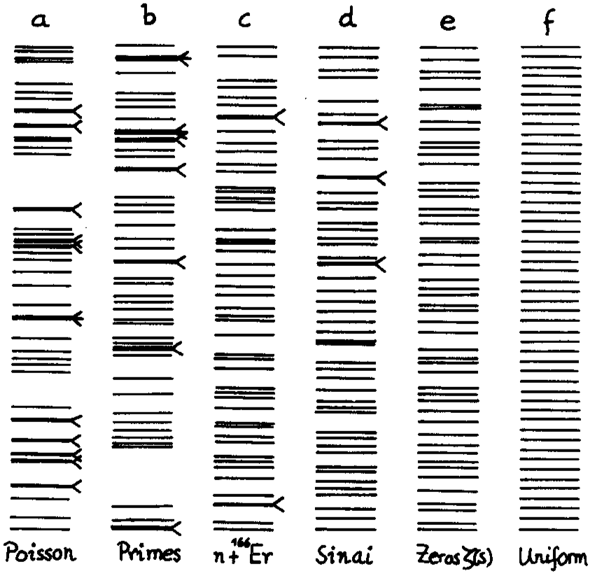
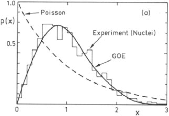
Typical distributions: Poisson, prime numbers, energy levels of an atomic nucleus, quantum Sinai billard, zeroes of the Riemann zeta function, and uniform. Histogram of the level spacings recorded from nuclear data compared to the random matrix gaussian orthogonal ensemble (GOE) and Poisson. From Bohigas and Giannoni (1984) and Bohigas et al. (1985).

It is important to note that for a subsystem to be in a well defined thermodynamic state, we do not need the whole system to be in the same thermodynamic state; the whole system, being completely isolated, can be for instance in a quantum pure state (and then not at all at equilibrium). This is possible because the thermodynamical state refers to local observables, whose quantum expected value (computed with the appropriated energy eigenvectors) will be equivalent to the one predicted by a statistical ensemble expectation value. This statement, already mentioned by Landau and Lifshitz in their book on statistics, is now known as the “eigenvector thermalization hypothesis” (see reference [DA]).

One may ask about the conditions under which local observables of a system have thermal expected values. A generic condition for the applicability of statistics is chaos.

Chaos is related to the emergence of statistical properties in otherwise deterministic systems; in classical systems it manifests by an extreme (exponential) sensitivity of particle trajectories on slight differences in the initial conditions (the Sinai’s billiard is a paradigmatic example); in quantum systems, where the notion of trajectory is precluded by the uncertainty principle, it is related to the statistical properties of the hamiltonian spectrum (atomic nuclei spectra or the quantum version of the Sinai billiard, are examples). See the lectures on chaos and reference [S].

Let us consider for simplicity an isolated system in a pure state \(\ket{\psi}\),

where \(\psi_n\) are the complex amplitudes in the energy basis \(\ket{n}\) of the hamiltonian \(H\). The expected value of a measurable operator \(M\) (a few body local operator, for instance), is at time \(t\), given by,

In order to obtain from this general (exact) equation the thermodynamic expected value in the microcanonical ensemble,

where \(\rho_E\) is the density matrix given by (\(\ref{micro}\)), it is necessary that (i) the first term be independent of the arbitrary initial amplitudes defining the whole system pure state \(|\psi_n|^2\),

(we used the normalization condition, \(\sum_n |\psi_n|^2= 1\)) for some typical \(n_E\) near the energy \(E\); and that (ii) the second term vanishes in the thermodynamic limit.

The first condition means that the diagonal elements of the observable \(M\) in the energy basis, are a smooth function of the energy, thus can be extracted from the sum which contains terms around \(E\), inside the relevant energy shell of width \(\Delta\). This is essentially the contents of the “eigenvector thermal hypothesis”:

for a closed quantum system.

The second condition supposes first that there is no significant degeneracy of the energy spectrum. In addition, it is a condition on the amplitudes of fluctuations around the dominant term (\(\ref{nn}\)).

Both conditions can be demonstrated to be a consequence of the statistical properties associated to the energy spectrum of a chaotic \(H\), which should be equivalent to the statistical properties of a random matrix hamiltonian. Now, as a special case, this should also be true in the semiclassical limit regime of classically chaotic dynamical systems. As a matter of fact, the eigenvectors of a random matrix are gaussianly distributed, one can therefore use the laws of large numbers and the central limit theorem to show that the mean of an operator is dominated by the diagonal terms (condition i) and that the fluctuations around the mean rapidly decrease (condition ii) with the dimension of the matrix (the number of degrees of freedom).

Experimental verification of the eigenstate thermalization hypothesis

Kaufman et al. (2016)[KL] experimentally tested the thermalization of the local observables of an isolated quantum system. They prepared a Bose-Einstein condensate of rubidium atoms in the form of a two-dimensional lattice. Initially the atoms were in a product pure state (without entanglement). After a well controlled quench leading the system towards a high energy state, the interactions between the bosons dynamically generate entanglement. The abstract of their paper reads:

Statistical mechanics relies on the maximization of entropy in a system at thermal equilibrium. However, an isolated quantum many-body system initialized in a pure state remains pure during Schrödinger evolution, and in this sense it has static, zero entropy. We experimentally studied the emergence of statistical mechanics in a quantum state and observed the fundamental role of quantum entanglement in facilitating this emergence. Microscopy of an evolving quantum system indicates that the full quantum state remains pure, whereas thermalization occurs on a local scale. We directly measured entanglement entropy, which assumes the role of the thermal entropy in thermalization. The entanglement creates local entropy that validates the use of statistical physics for local observables. Our measurements are consistent with the eigenstate thermalization hypothesis.

In particular, they compared the thermodynamical (in the canononical ensemble) and the measured value of the so-called “purity” of the system

related to the Rény entropy with \(n = 2\):

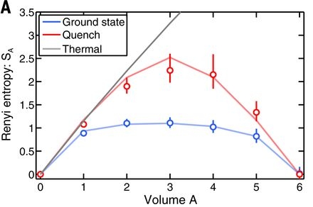
(it coincides with the von Neumann entropy for \(n = 1\)) where \(\rho_A\) and \(V_A\) are the state and the volume of subsystem \(A\). This quantity is largely insensitive to the system size when it is in its ground state, and is proportional to the volume in the thermodynamic case. They found that the experiment reproduces these predictions, demonstrating in addition the relation between entanglement and thermodynamic entropy (figure below).

Experimental measurements of the second Rény entropy \(S_2\) as a function of the subsystem volume \(V_A\). The black staight line is the thermodynamic canonical (Rény) entropy as predicted by statistical physics theory at a temperature corresponding to the mean value of the system’s energy (after the quench). The red line corresponds to the quenched state \(\rho_A\), and the blue line to the ground state. The initial growth of the entropy in the case of the high energy state (red), match the thermodynamic prediction (black); the subsequent bending results from the finite size (here 6 particles) of the subsystem A. The global state of the system is pure, as confirmed by the vanishing of the entanglement at \(V_A = 6\). One observes that the ground state entropy is only slightly dependent on the volume, result also consitent with the theoretical predictions. [Kaufman et al. (2016)]

Notes

References

[DA] D’Alessio, Kafri, Polkovnikov and Rigol, “From quantum chaos and eigenstate thermalization to statistical mechanics and thermodynamics”, Advances in Physics, 65, 239 (2016) (.pdf)

[K] Kadanoff, “Statistical Physics: Statics, Dynamics and Renormalization” (Singapore, 2000)

[LL] Landau and Lifshitz, “Statistical Physics” (Oxford, 1980)

[NC] Nielsen and Chuang, “Quantum Computation and Quantum Information” (Cambridge, 2010).

[P] Peres, “Quantum Theory: Concepts and Methods” (Kluwer, 2002)

[SW] Schumacher and Westmoreland, “Quantum Processes, Systems and Information” (Cambridge, 2010)

[S] Stöckmann, “Quantum chaos” (Cambridge, 1999)

[KL] Kaufman, AM, ME Tai, A Lukin, M Rispoli, R Schittko, PM Preiss, and M Greiner, Quantum Thermalization through Entanglement in an Isolated Many-Body System, Science 353, 794–800 (2016)(.pdf)

Bibliography

• Landau, D. and Lifshitz, E., Statistical Physics (Pergamon Oxford, 1980). The classical text on statistical physics.
• Schwabl, F., Statistical Mechanics (Springer, 2006). Concise presentation of the basis of statistical physics. This book, primary addressed to undergraduate students, deals with more advanced subjects through well chosen applications.
• Kardar, M., Statistical Physics, vol. 1 Particles, vol. 2 Fields (Cambridge, 2007). Clear presentation, interesting applications.
• Sethna, J. P., Statistical Mechanics, Entropy, Order Parameter and Complexity (Oxford, 2021). Very interesting and up to date text with a wealth of applications; intermediate level.

Footnotes