\(\newcommand{\I}{\mathrm{i}} \newcommand{\E}{\mathrm{e}} \newcommand{\D}{\mathop{}\!\mathrm{d}} \newcommand{\bra}[1]{\langle{#1}|} \newcommand{\ket}[1]{|{#1}\rangle} \newcommand{\braket}[1]{\langle{#1}\rangle} \newcommand{\bbraket}[1]{\langle\!\langle{#1}\rangle\!\rangle} \newcommand{\bm}{\boldsymbol}\)

Lectures on statistical mechanics.

Solids: effective models

Solid is an ordered state of matter characterized by a crystal structure and electronic bands. Atoms are located on the sites of the crystal lattice, tightly bound to their neighbors, their vibrations give raise to phonons, the quantum of the acoustic modes; electrons, depending on the chemical properties of the atoms, can jump from one site to another, carry a magnetic moment (spin), or interact with the nucleus and crystal potentials through the spin-orbit coupling, giving rise to a wealth of different physical properties and effects, such thermal or electric conductivity, ferromagnetism, piezoelectric effects, quantum Hall conductance, giant magnetoresitence or topological effects. In spite of the complexity of the solid’s band structure, specific electronic properties can be described by relatively simple effective hamiltonians comprising a few parameters, in which the complex crystal structure is replaced by a regular lattice and the collective electron coulomb interactions, by short range neighbors interactions.

The simplest example is a free electron in a metal. The presence of the crystal periodic potential creates gaps in the continuum spectrum. A tight binding hamiltonian on a cubic lattice, in which the electron can jump from one site to one of its six neighbors, is enough to account for the band structure; the hoping energy \(t\) is the only parameter of the model:

where \(\boldsymbol y = \{ (x \pm 1,y,z), (x,y\pm1,z), (x,y,z\pm1) \}\), is a neighbor of the site \(\boldsymbol x \in \mathbb{Z}^3\) of the cubic lattice. The operator \(c({\boldsymbol x})\) annihilate the particle at site \(\boldsymbol x\):

its hermitian conjugate \(c^\dagger({\boldsymbol x})\), creates a particle at this site.

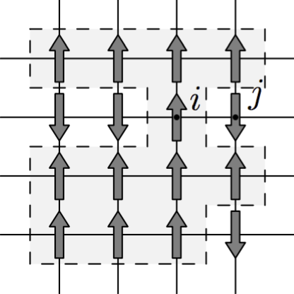
Many universal properties of magnetic systems are well described by the ising hamiltonian,

where \(s_{\boldsymbol x} = \pm 1\) is a classical spin variable, \(J\) is the exchange energy constant, and \((\boldsymbol x, \boldsymbol y)\) are neighboring sites in a lattice. The ising model is a simplified version of the quantum heisenberg hamiltonian:

where \(\sigma\) is the vector of pauli matrices. The ising and heisenberg hamiltonians, describe a magnetic material as a set of spins (classical or quantum), attached to the sites of a lattice (linear, square or cubic, depending on the dimension, for example), interacting with their nearest neighbors via the \(J\) exchange coupling (mimicking the overlap of electronic functions).

Ising model of a ferromagnetic material. Two dimensional lattice of interacting neighboring spins. The gray region defines a cluster of up spins.

More generally, lattice models are useful in a variety of domains, ranging from condensed matter to biology or social sciences. They can describe statistical equilibrium properties, like phase transitions, or nonequilibrium processes, like crystal growth,¹ population dynamics in a living system,³ or opinion propagation in a social network.²

Free particles in a lattice

We consider a gas of noninteracting, spinless bosons in a cubic lattice of step size \(a=1\), which we take as the length unit (fermions can be treated similarly). The system’s hamiltonian is,

where \(N\) is the number of particles and the operators create or annihilate particle \(n\) at a lattice site \(\boldsymbol x \in \mathbb{Z}^3\). In order to write the grand potential we diagonalize the hamiltonian using a change of the position basis \(\boldsymbol x\), to the momentum \(\boldsymbol k\) basis, through the fourier transformation,

where \(V=L^3\) is the number of sites in the cubic lattice of edge \(L\), the integration is over the first “brillouin zone” (here, the cube \(\mathrm{BZ} = (-\pi,\pi)^3\) in momentum space). Note that the inverse transformation gives,

and that,

is the kronecker delta. In the momentum basis the hamiltonian becomes EX,

where

Comparing this formula with the one of a free particle one finds that \(t \sim \hbar^2/2ma^2 \rightarrow \infty\)

The grand potential \(\Phi(T,\mu,V)\) of the noninteracting hamiltonian, writes:

where \(H\) is the single particle hamiltonian. The number of particles and the energy are given by the integrals,

and

To compare the behavior of the gas in a lattice with the ideal gas, we keep the first term in the fugacity (Boltzmann limit, which is similar for fermions and bosons). In this limit we have,

where \(I_0\) is the modified bessel function of the first kind,

and the particle number,

which combined with the expression of \(\Phi= -PV\), one recovers

independent of the hoping energy \(t\). However, the lattice gas energy differs from the one of the ideal gas.

Indeed, the energy is given by,

or, eliminating the chemical potential,

In the limit dominated by the kinetic energy \(T \ll t\), \(E\) approximates EX,

where the second term corresponds to the ideal gas result (the first term, a constant independent of the temperature, do not contribute to the specific heat, can be eliminated by a shift of the zero of the energy). We used the asymptotic expression,

In the opposite limit \(T \gg t\), the energy grows slowly with the temperature:

which gives a specific heat decreasing at high temperature, behavior consistent with the exponentially low probability of jumps. (The small \(z\) limit of the \(I\) bessel functions is \(I_n(z) = (z/2)^n/n!\).)

One dimensional spin model

In the presence of an external field \(B\), the one dimensional ising hamiltonian is,

where we assumed periodic boundary conditions \(s_1 = s_{N+1}\). We choose units based on the lattice constant and the spin magnetic moment, \(a = g\mu_\text{B}=1\) (we also put the permeability \(\mu_0=1\)); in such units the magnetic field \(B\) has the dimensions of the energy.

The probability of a spin configuration \(s\),

is,

and the partition function is given by,

where \(K = J/T\). We observe that the thermodynamics of the present model depends on two nondimensional parameters, the interaction energy-temperature ratio \(K = J/T\) and the external field-temperature ratio \(h = B/T\). The idea to compute the partition function is to try (obviously this is not always possible) to factor it in a series of identical terms, like in the noninteracting case; we symmetrized the \(B\) term to this goal. We note first that the product appearing in \(Z\) can be written in the form,

where each term \(T_{s_x,s_{y}} = T_{s_y,s_x}\) can take different values according to the values of \(s_x = \pm 1\) and \(s_{y} = \pm 1\):

Therefore, the partition function becomes,

A generic factor is,

corresponding to the product of two matrices,

Using the transfer matrix \(T\) to write the partition function,

Therefore, using the invariance of the trace under basis transformations EX,

where \(\lambda_\pm\) are the eigenvalues of the transfer matrix \(T\):

In the thermodynamic limit \(N\rightarrow\infty\), only the larger eigenvalue of the transfer matrix survives in \(Z\):

from which we compute the free energy,

The mean magnetization per particle \(m=M/N \braket{s_x}\), is given by EX,

In the limit of small \(B\) (and finite temperature), the magnetization is proportional to the field:

a behavior of the paramagnetic type, with a susceptibility inversely proportional to the temperature, corrected with the factor \(\E^{J/T}\) depending on the interaction energy. However, for \(T=0\), te magnetization becomes,

behavior reminiscent to a phase transition (at critical temperature \(T_c=0\)): indeed, at zero temperature the two values of the magnetization \(m=\pm1\) correspond to an ordered state with all spins pointing up or down.

The correlation function (at \(B=0\)) between two spins separated by a distance \(r\), is defined by,

We introduce as before, the transfer matrix \(T\),

which gives, using the matrix product formula,

Using now the unitary transformation,

to diagonalize \(T\), and the cyclic property of the trace \(\mathrm{Tr}\, ABC = \mathrm{Tr}\, (U^\dagger A U)( U^\dagger B U)( U^\dagger C U)\), we obtain EX,

Therefore the two spins correlation function of a Ising system with \(N\) spins is given by the explicit formula,

In the thermodynamic limit \(N \rightarrow \infty\), we finally get,

where \(\xi\) is the correlation length. The exponential decay of correlations indicates the absence of long range order. The 1D Ising model has not phase transitions for \(T>0\).

Mean field spin model

Instead of considering the nearest neighbor interaction, we can investigate the case of long range interaction, where each spin on a lattice indexed by \(x=1,2,\ldots,N\) (\(N\) is the number of spins) can interact with all other spins:

where the factor two is to avoid counting twice each pair \((x,y)\), and the factor \(1/N\) is to ensure that the energy is extensive (there are \(\sim N^2\) terms of order one in the sum). This model is easily solved by noting that the hamiltonian corresponds to one spin in an effective field \(B_s\) created by the other spins, in addition to the real applied field:

where

is the magnetization per site, or, inserting this expression into \(H\),

The partition function is then,

the free energy is,

and the magnetization is given by the self-consistent equation,

At variance to the one dimensional case, the mean free model account for the existence of a non zero magnetization, even in the absence of an external magnetic field. Such a state is called ferromagnetic: it is a thermodynamic phase with ordered spins and spontaneous magnetization; it differs to the disordered paramagnetic phase, whose spontaneous magnetization vanishes. Therefore, the mean field model is able to describe a magnetic system undergoing, as a function of the temperature and magnetic field, a phase transition from a disordered state at high temperatures, to an ordered state at low temperatures. The critical temperature is given by \(T_c=J\). For \(T > T_c\), only the value \(m = m_P(T) = 0\) is solution, while for \(T,T_c\) two equilibrium values are found \(m = \pm m_F(T)\), corresponding to the paramagnetic and ferromagnetic phases respectively.

Let us compute the heat capacity and the susceptibility in the present framework. Calculating the derivative of the free energy with respect to the temperature we find the energy EX,

in the form of an implicit function of the temperature, through the equilibrium value of the magnetization (\(m_P\) or \(\pm m_F\)). The derivative of \(E\) with respect to \(T\) gives the specific heat,

where we used the expression of the derivative,

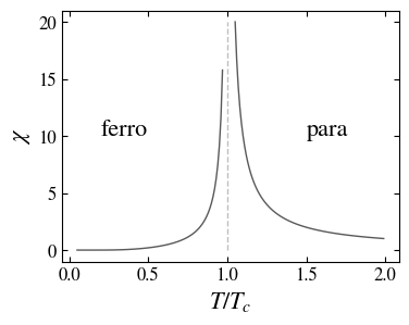
The susceptibility is computed using also the derivative of the implicit function \(m=m(T)\),

at \(B=0\).

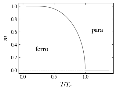
Magnetization and susceptibility as a function of the temperature (\(B=0\)). A phase transition occurs at \(T=T_c\) between a height temperature disordered state \(m=0\) (paramagnetic) and a low temperature ordered state \(m \ne 0\) (ferromagnetic); at the transition temperature the susceptibility diverges.

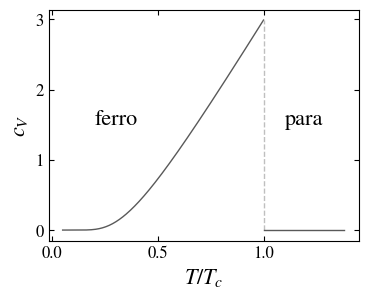
The specific heat (at zero magnetic field),

presents a discontinuity at the critical temperature. This behavior is specific of the mean field approximation, more realistic models give a divergence of the form,

characterized by the exponent \(\alpha\).

Specific heat capacity of the ferromagnet as a function of the temperature; at the critical temperature it has a jump of \(3\). In the paramagnetic state the specific heat of the magnet vanishes.

Monte Carlo method

Second order phase transitions arise in magnetic materials, superfluids, superconductors, liquid crystals, and solid allows; although microscopically different, they are described by the same critical exponents: they are examples of order-disorder transitions.

The study of critical properties of physical systems near a phase transition relies, for a large part, on numerical simulation:

• Monte Carlo methods: allow the investigation of (classical and quantum) equilibrium systems.
• Kinetic Monte Carlo: suitable for nonequilibrium systems
• Molecular dynamics: used in soft matter (liquids, polymers)

Monte Carlo methods are based on a Markovian process, they reject or retain a given modification in the state of a system at each step, provided the change optimize some suitable functional (the energy, for a mechanical system; the Gibbs distribution, for a thermodynamic system)

The dynamics of weakly nonequilibrium systems, well approximated by a Markovian process, or systems relaxing towards the equilibrium, is described by a master equation. It gives the probability \(P\) that a system \(S\) be at state \(s\) at time \(t+1\) given its state at \(t\) is the same \(s\) or other possible configuration \(s'\),

where \(T\) is the transition probability between states \(s\) and \(s'\), not necessarily equivalent in the two directions. The sum is over all possible configurations of the system, \(s' \ne s\). At the stationary state the right hand side must vanish. A sufficient condition is,

which is called detailed balance

The Metropolis method, uses the thermodynamic equilibrium Gibbs distribution as the stationary probability distribution,

(\(\beta\) is the usual notation of the inverse temperature). It is convenient to write the transition probability in the form \(T(s \rightarrow s') = w_s A_{ss'}\), where:

• \(w\) is the trial step probability, for the ising system this is the probability to choose a random site in the lattice and change its spin
• and \(A\) is the acceptance probability
  $$\frac{A_{ss'}}{A_{s's}} = \frac{P(s')}{P(s)} = \E^{\beta E(s) - \beta E(s')}$$
  one has,
  $$\frac{T(s \rightarrow s')}{T(s' \rightarrow s)} = \frac{w_{s}}{w_{s'}} \frac{A_{ss'}}{A_{s's}}= \frac{P(s')}{P(s)}$$
  where we assumed symmetric trials \(w_{s}= w_{s'}\).

The metropolis algorithm proceeds in two steps: given a configuration \(s\)

• we choose a new configuration \(s'\) with probability \(w_{s}\)
• if the probability of this configuration satisfies \(P(s') > P(s)\) then we accept the new configuration
  $$A_{ss'} = 1,\ \text{if } P(s') \ge P(s)$$
  otherwise, we put
  $$A_{ss'} = \frac{P(s')}{P(s)} ,\ \text{if } P(s') < P(s)$$
  and accepts \(s'\) with probability \(A_{ss'}\), in summary:
  $$A_{ss'} = \min[1, P(s')/P(s)]$$

This algorithm ensures that the detailed balance condition is satisfied and that the asymptotic, stationary, probability distribution is the Gibbs distribution at the given temperature.

In the metropolis algorithm only one spin at each step is reversed; near the transition, where the spins are in large patches having the same orientation (clusters), the rejection probability is large. To remedy at this, simultaneous reversal of many spins is much more efficient. This is the idea of the Wolff cluster algorithm.

At variance to the metropolis algorithm which supposed the trial probability independent on the configuration, let us assume that \(w_s \ne w_{s'}\). The condition of detailed balance becomes,

For the construction of the cluster we must specify in addition to the Gibbs weights, the rules of accepting or rejecting the configuration.

Let us consider a \(s=1\) cluster \(C\); there are \(n_1\) pairs \((1,1)\) and \(n_2\) pairs \((1,-1)\) at its border \(\partial C\). The contribution of the border to the energy is

(in units of the exchange constant \(J=1\)). The gibbs probability of the \(s\) spin configuration, is then

If \(p\) is the probability to add a site to the cluster, we can assume the form trial probability associated to \(s\), to be

which gives the a priori probability to stop growing the cluster \(s\) whose spins will be reversed (leading to a new configuration \(s'\)). Therefore, using similar rules to go back to the configuration \(s\) from \(s'\), the acceptance probability is given by the rule,

this means that with this special value of \(p\), once the cluster is formed, we reverse it with probability \(1\). It is the existence of this special value of \(p\), leading to full acceptance, that makes the algorithm particularly performant.

Numerical computation of the ising model

We consider the ising model in a square lattice of size \(L\),

(with \(J=1\) the energy unit and where the sum runs over the nearest neighbors) was exactly solved by Onsager (1944). It undergoes a ferromagnetic transition at the temperature

The magnetization per site \(m=\sum_x s_x/L^2\) is near \(1\) in the low temperature ferromagnetic state, and near \(0\) in the high temperature paramagnetic state. At the transition point the heat capacity

has a logarithmic cusp and the susceptibility

diverges as a power law with a characteristic exponent \(\gamma = 7/4\). The magnetization is given by the formula,

which gives, near the transition, also a power law with characteristic exponent \(\beta=1/8\) (the mean field gives \(\beta=1/2\)).

We use the monte carlo method to investigate the statistical properties of the ising system; here we gives, as an example, the two dimensional routines of the metropolis and cluster algorithms.

#
# Metropolis algorithm
#
def metropolis(s, kT):
    """
    Reference:
        Newman, M and Barkema, G., *Monte Carlo Mehtods
        in statistical physics* (Oxford, 1999), 
        Chap. 3 and p. 433.
    Input:
        s spin configuration
        temperature kT (in units of J)
    Output:
        new configuration s
    """
    L = shape(s)[0]
    flips = 0
    while flips <= L**2:
        (x, y) = (randint(L), randint(L))
        # compute energy required to flip spin
        dE = s[(x+1)%L,y] + s[(x-1)%L,y] + s[x,(y+1)%L] + s[x,(y-1)%L]
        dE *= 2.0*s[x,y]
        # Metropolis algorithm to see if we should accept trial
        if (dE <= 0.0) or (random.random() <= exp(-dE/kT)):
            # accept trial: reverse spin; return dE and dM
            s[x,y] *= -1
        flips += 1
    return s
# Energy and magnetization (one MC step)
def thermo(s):
    # Use: (M, E) = thermo(s)
    dE = s*(roll(s,1,axis=0) + roll(s,-1,axis=0) + 
              roll(s,1,axis=1) + roll(s,-1,axis=1))
    return sum(s), -sum(dE)/4

#
# Cluster algorithm
#
def flip_cluster(s, kT):
    """
    References:
        Wolff cluster algorithm, Phys. Rev. Lett. **62**, 361 (1985)
        Newman, M and Barkema, G., *Monte Carlo Mehtods
        in statistical physics* (Oxford, 1999), 
        Chap. 4.2 and p. 437.
    """
    p = 1.0 - exp(-2/kT)
    L = len(s)
    #
    flips = 0 # number of flips
    # sweep the lattice once
    while flips <= L**2:
        # initialize cluster on a random site
        (x, y) = (randint(L), randint(L))
        cluster = [(x, y)] # cluster stack
        s_in = s[x, y]
        s_out = -s[x, y] # and flip it
        s[x, y] = s_out
        flips += 1 # update count
        while cluster != []:
            # remove the first site of the cluster stack
            (x, y) = cluster.pop(0)
            # check neighbors for acceptance
            neighbors = [(x, (y+1)%L), ((x+1)%L, y),
                         (x, (y-1+L)%L), ((x-1+L)%L, y)]
            for site in neighbors:
                # is same sign?
                if s[site] == s_in:
                    # use the acceptance probability (temp)
                    if random.uniform(0,1) < p:
                        cluster.append(site)
                        s[site] = s_out
                        flips += 1 # update flips count
    return s

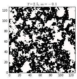
The figures below show magnetization snapshots of the two phases and at the transition.

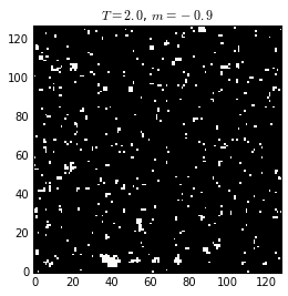
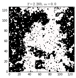
Spin configurations (black and white represent the two states at each lattice site) of a 2D ising system below, at, and above the critical temperature, \(T_c \approx 2.269\) (or \(\beta_c=0.4407\)). The critical state characterizes by the existence of ferromagnetic domains having any size, randomly distributed on the lattice. At lower temperature the ordered domain is of the size of the system. At higher temperature, the magnetization is randomly distributed, with zero mean.

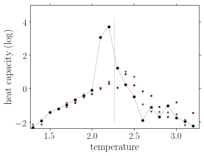
We can also compute the thermodynamic quantities, and observe their singular behavior at the transition. A quantitative comparison with the Onsager formulas can be made. In addition, the method can of course be generalized to take into account an external field, or to go to larger dimensions. In the three dimensional lattice (cubic lattice), the exponent characterizing the vanishing of the magnetization in the paramagnetic state is \(\beta \approx 0.326\).

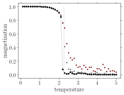
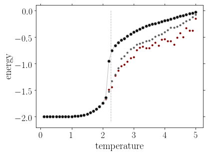
Magnetization, energy and heat capacity as a function of the temperature for the 2D ising model, from cluster monte carlo simulations. The heat capacity is shown in the region of the phase transition in a logarithmic scale. The three set of data correspond to \(L=20\) (red), \(L=64\) (gray), and \(L=128\) (black), to emphasize the finite size effect on the singularities present at the thermodynamic limit. The vertical line shows the critical temperature \(T_c=2.269\).

The XY model

Some twodimensional systems, like films of liquid helium, ferromagnets or superconducting materials, display a particular phase transition without low temperature order. In the general case second order phase transition are characterized by a low temperature ordered phase, like in a ferromagnet with develops a spontaneous magnetization, or the transition of liquid helium into a superfluid, and a disordered high temperature phase (paramagnetic state or normal liquid phase). One simple model undergoing the so called Kosterlitz-Thouless transition is given by a classical version of the heisengberg spin model:

where \(J=\bar{JS^2}\) is the characteristic coupling energy, and we sum overt the lattice points \(\bm x\) and its neighbors \(\bm y = \bm x + a \hat{\bm x}\) and \(\bm y = \bm x + a \hat{\bm y}\) (\(a\) is the lattice spacing). The interaction between two neighboring spins \(S_{\bm x}\) and \(S_{\bm y}\), where \(\bm x, \bm y\in \mathbb{Z}^2\) (the square lattice), reduces to their orientation difference \(\theta_{\bm x} - \theta_{\bm y}\). The classical model corresponds to a lattice of coupled “rotators”, whose degrees of freedom are their possible orientation. We observe that changing the angles by a constant \(\theta_{\bm x} \rightarrow \theta_{\bm x} + \theta_0\), do not change the hamiltonian; thus, \(\theta_0 \in (-\pi,\pi)\) is a continuous symmetry group parameter, at variance with the discrete symmetry characteristic of the ising model. The presence of a continuous symmetry precludes the existence of a second order phase transition (and a fortiori of higher order singular behavior). However, Kosterlitz and Thouless in a famous paper demonstrated that the correlations between spins separated by a certain distance behaves differently at low temperature, dominated by spin waves, and high temperature, dominated by vortices, a special kind of spin excitations. Our goal is to describe these two particular phases and investigate the nature of the phase transition.⁴

XY model: classical rotators in a square lattice; the degrees of freedom are the spin direction at each site \(\theta_{\bm x}\), and neighboring spins at \(\bm x\) and \(\bm y\), interact through the exchange coupling of strength \(J\).

We start by the low temperature behavior, in the region \(T \ll J\). The ground state of the system at \(T=0\) should be the one with fully aligned spins (note that \(\cos 0 = 1\) gives the weakest coupling); therefore, we expand the cosinus to get

At low temperature thus, neighboring spin are almost aligned that can be described by a smooth function \(\theta_{\bm x} \rightarrow \theta(\bm x)\) of the position \(\bm x \in \mathbb{R}^2\), a point in the plane; this replacement is valid if the characteristic length of the orientation gradients are much larger than the lattice length \(a\). In this continuum description we approximate the angle difference by the angle gradient:

where \(\bm a = a \hat{\bm x} + a \hat{\bm y}\). Within the same approximation, we replace the sum over lattice positions by an integral over the real plane,

Therefore, the effective low temperature hamiltonian reads,

Note that the lattice constant disappears: this is particular to the twodimensional case, in general dimension \(D\) the effective coupling constant would be \(J/a^{D-2}\). This hamiltonian accounts for the spin wave low temperature excitations above the ferromagnetic ground state. It is worth mentioning that the field \(\theta(\bm x)\) takes values in the interval \((-\pi, \pi)\), relaxing this constraint amounts at neglecting the multivaluedness of the field, and thus possible topological effects associated to this multivaluedness. We shall return to this important point later. Without topological constraint it is straightforward to compute the thermodynamic properties transforming the low temperature rotators into a field of harmonic oscillators. This can be done by fourier transforming the angle field:

Introducing this transformation into \(H\), we obtain

Or taking into account that \(\theta(\bm x)\) is real \(\theta_{-\bm k} = \theta^\star_{\bm k}\), giving

where we used the definition of the kronecker delta:

in which we suppose \(\bm k\) to be dimensionless and put \(\bm x\) explicitly in units of \(a\), to identify the behavior when \(a \rightarrow 0\). We write the complex field \(\theta_{\bm k} = a_{\bm k} + \I b_{\bm k}\) in terms of the real fields \(a_{\bm k}\) and \(b_{\bm k}\), to obtain

Therefore, in fourier space the hamiltonian is diagonal with eigenvalues,

which is the dispersion relation of ferromagnetic spin waves in the long wavelength limit (in two dimensions).

To characterize the spin waves we need to go further than the mere mean value \(\braket{\theta}\), which can only assesses the global orientation (in fact, \(\braket{\cos \theta_{\bm x}} = 0\) vanishes for all temperatures EX); we need instead to know the behavior of the rotators separated by a given distance. The natural quantity measuring the mutual influence of two distant rotators is their correlation function, which we define by the formula

or equivalently,

where we used the translation symmetry (the field is homogeneous, their properties do not depend on the origin of coordinates). The mean is computed with respect to the canonical probability distribution:

which depends on the configurations of the field \(\theta_{\bm k}\).

We note that a gaussian random variable \(x\) satisfies:

Using this formula we rewrite the correlation function in a simpler form,

We must thus compute

where \(Z\) is the partition function. The integral span all the degrees of freedom in fourier space (equal to the number of sites in the lattice \(N\)). The last factor is readily transformed in fourier space:

we separate the diagonal terms \(\bm k_1 + \bm k_2 = 0\),

to obtain,

where the second non diagonal term factorises into a product whose average vanishes because \(\braket{\theta_{\bm k}}=0\) (the gaussian integral of an odd function is zero). The mean of each term in the sum is of the form,

where

Putting this result into the correlation function we obtain,

This expression is valid for small \(k\), therefore we can replace the sum by an integral

Using \(\bm k \cdot \bm x = kr \cos(\varphi)\) and the definition of the zero order bessel function

the sum is approximated, after integration over the polar angle \(\varphi\), by

Note the upper value of the integral, where we introduced the cutoff \(\pi/a\) which is the maximum value of the wavenumber compatible with the finite number of degrees of freedom (using the fact that at large distances \(r \gg a\) the lattice is isotropic —as evidenced by the form of the spin wave hamiltonian which depends on the square of the gradient). The integral is then dominated by its value at the upper limit (it is regular at 0):

Therefore, we arrive at the final expression of the two spin correlation function:

This is an important result. We observe that at low temperature the spin correlation function decreases algebraically. This slow decay is an indication of a kind of long range order, however, the characteristic exponent depends on the temperature. Before fully discussing this result, we should investigate the high temperature regime.

Path between spins at \(\bm x\) and \(\bm y\) contributing to the high temperature correlation function.

For \(T \gg J\) the correlation (returning to the lattice notation)

or using \(J/T \ll 1\) we expand the exponential

We note, on the one hand, that any term with single bond vanishes,

on the other hand, two successive bonds

The first condition leads to the conclusions that the only contribution to the correlation function are paths of bonds emanating from \(\bm 0\) and reaching \(\bm r\):

as represented in the figure. Analogously, the contribution of the end points

Each intermediate term of the path contributes a factor \(J/2T\) (corresponding to the second integral). Therefore, at high temperature the dominant contribution comes from the shortest path, the one with the smaller number of \(J/\) factors:

because \(r/a\) is the number of links in the path between \(\bm 0\) and \(\bm r\). We finally obtained that at high temperature the correlations decay exponentially fast; the characteristic length depends on the temperature,

Then, gathering the high and low temperature results together, the following picture arises. The system is disordered at high temperature, in the same way of a paramagnetic material; at low temperature it shows a critical behavior characterized by algebraically decaying correlations. The mean of a critical state is related to the absence of characteristic length; one may find patches of aligned rotators at all scales, like in the critical region (around a phase transition) of the ising model, as we observed in the monte carlo simulations (previous section).

A question naturally arises about the mechanism driving the transition between these two qualitatively distinct physical regimes. Kosterlitz and Thouless⁵ demonstrated that it is the unbinding of vortices, a particular kind of excitations different to the spin waves prevailing at low temperature. The idea is that in addition to spin waves other, finite energy excitations can exists. Vortices are topologically nontrivial configurations of a vector field, textures that cannot be continuously deformed into a, say, constant field. In two dimensions the simplest vortex configuration is (in the continuous approximation),

which, as a consequence of the angle periodicity, the circulation satisfies,

implying that \(q\) must be an integer, and is called the vortex charge (correspondign to the topological charge or, in the present case, the field \(\bm v\) winding number); the closed path in the plane \(\mathcal{C}\) is arbitrary. The discrete version of the previous integral is,

The energy of a vortex of charge \(q\) is

or

and we introduced the short and long lengths cutoffs, the lattice step \(a\), and the system’s size \(L\), respectively. The corresponding entropy can be estimated form the number of configurations one vortex can take in a system of size \(L^2\); taking into account that the vortex core occupies one plaquette of size \(a^2\), the number of configuration is \(L^2/a^2\):

The free energy of a vortex is,

Therefore, we have vortex excitations that, as a result of the logarithmic energy and entropy increase with the system’s size, their free energy change sign at a critical temperature

above the Kosterlitz-Thouless temperature \(T > T_{KT}\), the one vortex free energy is negative, meaning that increasing the number of vortices we can lower \(F\); under \(T_{KT}\) (\(T< T_{KT}\)), the free energy is positive and vortices become thermodynamically unfavorable. Thus, \(T_{KT}\) separates a low temperature phase in which there are not free vortices (in fact vortices are bounded in pairs), and a high temperature phase dominated by free vortices.

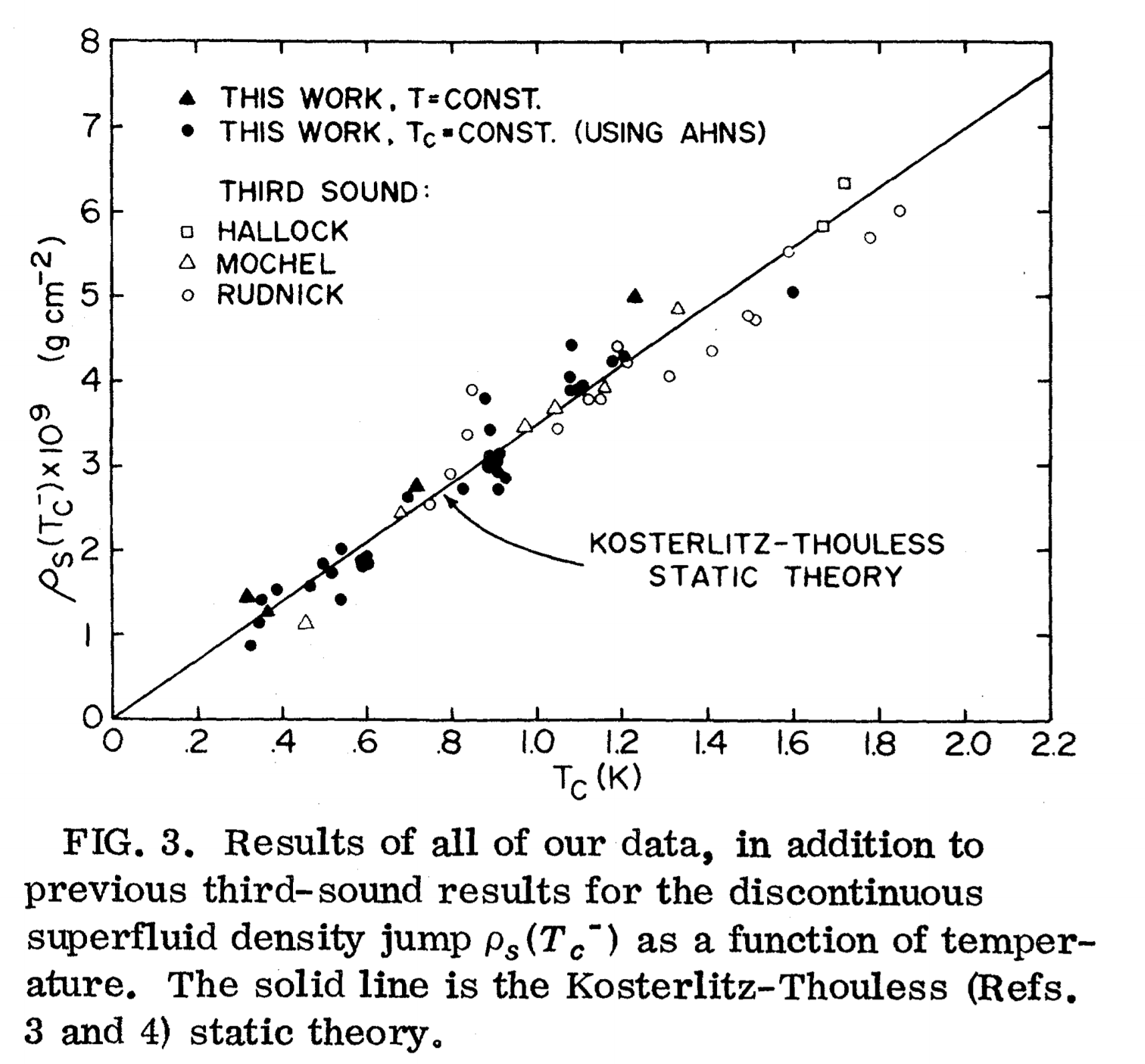
Experimental measure of the superfluid mass per unit area \(\rho_s\) as a function of the critical temperature: the Kosterlitz-Thouless theory predicts a universal constant, given by the slope of the straight line (equivalent to the relation \(T_{KT}/J = \pi/2\) in the XY model); by Bishop and Reppy, Study of the Superfluid Transition in Two-Dimensional \(^{4}\mathrm{He}\) Films, Phys. Rev. Lett. 40, 1727 (1978) ©1978 American Physical Society.

The fact that at low temperature vortices are bounded results form their finite interaction energy EX:⁴

where \(q_1\) and \(q_2\) are their charges, and \(|\bm x - \bm y|\) is their separation. Therefore, lowering the temperature free vortices tend to form pairs with other vortices (note that the total vortex charge must vanish).

Snapshot of the XY rotators at a temperature above the transition temperature \(T_{KT}\), showing many pairs of vortices (\(q=1\) in red \(+\), and \(q=-1\) in blue \(\times\)), and some isolated vortices (gray circles). Only a lattice sector \(16 \times 16\) is shown.

The high and low temperature expansions showed that the XY model, even if it lacks of an ordered ferromagnetic-like phase, exhibit a kind of long range order below some critical temperature; however, the precise description of the transition, viewed as the unbinding of vortex (topological) excitations, needs an account of the vortex interaction. The vortices can be seen as a gas of charged particles interacting through a coulomb potential, proportional to the logarithm of the distance between two charges in two dimensions; the collective action of this potential is to screen a test charge (as in a real plasma), modifying the “dielectric” properties of the medium. Kosterlitz and Thouless, using the model of a two dimensional coulomb gas, derived the critical properties of the XY model. Within this analogy the transition appears as the transition between an isolating state, in which the charges (vortices) are bounded, to a metal state in which they are free. The method to investigate the critical behavior in interacting systems is the renormalization group. It allows the investigation of the influence of the short scales, of the order of the lattice spacing \(a\): a change in \(a\) renormalize the effective interaction of the vortices \(J\). Beyond the spin wave approximation, the effect of the interactions can be encoded in an effective scale dependent coupling parameter \(J \rightarrow J(a)\). This can be illustrated by considering the partition function of a single vortex (we put \(q=1\)),

where \(\epsilon_0(a)\) is the vortex selfenergy (the energy necessary to create a vortex). If we change \(a\) into \(ba\) (\(b\) is then a scale factor) and impose that the partition function do not change we get EX,

showing that a change of scale modifies the vortex core energy, and thus their effective interaction, which becomes scale dependent \(J \rightarrow J(b)\), as anticipated before. The invariance of the thermodynamic properties, which cannot depend on the scale factor, leads to a set of renormalization equations for the parameters \(y_0(b)\) and \(J(b)\). Finding the fixed point of these equation (a further change of scale, do not change the solution) leads to explicit expressions of the critical temperature (correcting the previous estimation using the one vortex free energy)

giving a critical temperature below the bare value \(\pi/2\), the correlation length,

and free energy in the critical region:

where \(c\) is a numerical constant (\(c\approx 1.5\)). Therefore, the free energy has an essential singularity at the transition point, leading to continuous thermodynamic quantities (its derivatives are continuous functions of the temperature across the transition); in this sense we can say that the Kosterlitz-Thouless transition is of infinite order.

Notes