$\newcommand{\I}{\mathrm{i}} \newcommand{\E}{\mathrm{e}} \newcommand{\D}{\mathop{}\!\mathrm{d}} \newcommand{\Di}[1]{\mathop{}\!\mathrm{d}#1\,} \newcommand{\Dd}[1]{\frac{\mathop{}\!\mathrm{d}}{\mathop{}\!\mathrm{d}#1}} \newcommand{\bra}[1]{\langle{#1}|} \newcommand{\ket}[1]{|{#1}\rangle} \newcommand{\braket}[1]{\langle{#1}\rangle} \newcommand{\bbraket}[1]{\langle\!\langle{#1}\rangle\!\rangle} \newcommand{\bm}{\boldsymbol}$

Lectures on statistical mechanics.

Phase transitions

The thermodynamic state of a system can be described by a general free energy $F=F(K)$, which depends on a set $K$ of intensive and extensive variables, such as, the temperature, volume and particle number $T,V,N$, the magnetization $M$, the applied external magnetic field $H$, or more generally, the set of parameters appearing in the microscopic hamiltonian: characteristic lengths of the interaction, magnetic exchange energies, spin-orbit coupling, etc. The free energy is a continuous convex up (concave) function of its arguments, as can be derived from its definition in statistical mechanics,

$$ F = - T \ln Z $$

(we take $k_\mathrm{B}=1$, as usual) where the canonical partition function $Z$ is essentially a sum of exponentials.

A thermodynamic phase is the region in parameter space $K$ (the thermodynamic phase space) where $f=F/V = f(K)$, in the thermodynamic limit, remains analytic ($V, N \rightarrow \infty$), or in other terms, phases are homogeneous systems with stable qualitative physical properties. However, varying a parameter (for instance the temperature, or the external magnetic field), may induce a dramatic change in the state of the system. These changes signal the existence of a phase transition at a critical value of the control parameter. Common examples of phase transitions are the solid-liquid and para-ferromagnetic transition: lowering the temperature, the control parameter, one passes from a isotropic liquid to a cristalline solid, or from a disordered isotropic state (paramagnetic) to an ordered state (ferromagnetic) of lower symmetry.

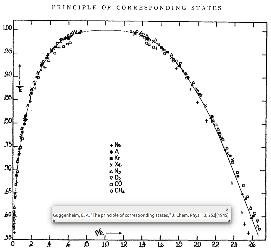
One may distinguish two types of transitions between different thermodynamic phases: phase transitions associated with a release or absorption of latent heat (first order in the Ehrenfest classification) characterized by the appearance of a discontinuity in the thermodynamic quantities; and continuous phase transitions (second order in the Ehrenfest classification; however, this terminology is not appropriated because, for instance, the heat capacity can diverge at the transition). Phase diagrams represent the different phases in the parameter space: the plots below are typical of argon, which behaves as other classical fluids, and helium (He), which undergoes a superfluid phase transition at around $4\,\mathrm{K}$ (the $\lambda$ line).

Typical phase diagram in the pressure-temperature space of a classical fluid (Ar) and of helium. First order transitions are double lines, second order ones simple lines. The transition line between gas and liquid phases ends at the critical point (PC); the three phases (solid-liquid-gas) join at the triple point. In the case of helium, the $\lambda$ line, starts and ends at points in which a second order phase transition transforms into a first order one. The superfluid phase is quantum; note that the liquid state remains up to zero temperature for a range of pressures.

The figures below show experimental data of the gas-liquid, a first order transition, and the second order, continuous, transition between disordered and ordered magnetic states.

Liquid-gas coexistence curve for different fluids showing a universal behavior near the critical point. The fitting solid line is a cubic interpolating polynomial, which leads to the power law for the density as a function of the temperature, $(\rho - \rho_g)/\rho_g \sim (T-T_c)^\beta$, with $\beta = 1/3$, near the transition temperature $T_c$. More accurate experimental results show that $\beta\approx 0.354$.

A distinctive property of (continuous) phase transitions is their universal behavior. Indeed, the thermodynamic quantities at the critical control parameter, follow power laws with universal exponents, exponents that do no depend on the details of the material or on the specific form of the microscopic interaction forces. This is the case, as discovered by Widom, of the equation of state of a magnetic material $H=H(M,T)$ relating the magnetic field $H$ to the magnetization $M$ and the temperature $T$, which, around the transition, can be written in the similarity form,

$$ H = M^\delta g(t/M^\beta)\,, \quad t = |T-T_c|/T_c\,, $$

thus, the two variable function $H(M,T)$ collapses into a “universal” single variable function characterized be the exponents $\beta$, which controls the temperature dependence of the magnetization, and $\delta$, which gives the behavior of the magnetization as a function of the applied field at $t=0$. Different ferromagnetic materials (Fe, Ni, Co,…), as experimentally verified, satisfy this law with the same function $g$ (see the figure below).

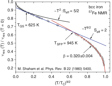
Iron magnetization as a function of the temperature $T^{9/2}$, showing the scaling exponent $\beta = 0.3$ typical of the 3D ising universality class. Other exponents shown characterize various quantum transitions at relatively low temperatures [Köbler and Hoser (2010)]

In the paramagnetic state the macroscopic magnetization $\bm M$ vanishes. The magnetization is defined as the thermodynamic average of the microscopic magnetic moments $\bm \mu$ per volume unit,

$$ \bm M = \frac{1}{V} \sum_x \braket{\bm \mu_x}\,, $$

for a homogeneous state, where the magnetic moment is related to the spin by $\bm \mu = -g\mu_B \bm S$ ($\mu_B$ is the Bohr magneton and $g$ the g-factor). In the ferromagnetic state, the magnetization acquires a nonzero value together with a definite direction, even in the absence of an external magnetic field. Although the behavior of the magnetization at low temperature is rather complex, because of the appearance of quantum effects, near the transition the magnetic properties are the same for a variety of ferromagnetic materials, and characterized by a unique exponent $\beta \approx 0.3$. However, some other materials, such us the gadolinium-zinc, also follows a power law, but with a different exponent, $\beta = 1/2$, which corresponds to the “mean field” value, as we shall see (figure below).

Magnetization square as a function of the temperature near the critical temperature, showing the power law $m\sim (T_c - T)^\beta$, with a scaling exponent $\beta = 1/2$, typical of the mean field theory of a ferromagnetic transition below the critical temperature $T_c$ [Köbler and Hoser (2010)]. The magnetic susceptibility is also displayed for $T>T_c \approx 270\,\mathrm{K}$, showing that the Curie law $\chi \sim (T-T_c)^{-1}$ is satisfied in the paramagnetic state, but with a divergence at $T_c$.

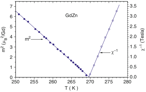
One important feature of the continuous phase transition is the presence of large fluctuations, leading to the divergence of the heat capacity (related to the fluctuation of the energy) and the susceptibility (related to the response to an applied external force). The figure above shows that the magnetic susceptibility near the transition, diverges following a power law,

$$ \chi = \left. \frac{\D M}{\D H} \right|_{H=0} \approx (T-T_c)^\gamma\,, $$

with exponent $\gamma$ (equal to $-1$ in the mean field case).

Landau theory of phase transitions

A defining property of the continuous phase transition is the difference in the symmetry of the states above and below the critical control parameter. This difference implies an essential discontinuity in the thermodynamic properties of the two phases: the symmetry exists or not. To describe the symmetry of the phases Landau introduced a thermodynamic variable, the order parameter $\phi$, which vanishes above the transition and, below the transition, it is nonzero. The mathematical nature of the order parameter depends on the physical properties of the system:

is a scalar $\phi = (p_A - p_b)/(p_A + p_B))$, where $p_A$ and $p_B$ are, in an alloy $AB$, the probabilities to find the respective atom in a given site of the crystal lattice, in the transition between two cristalline structures,
is a vector $\bm M$, the magnetization, in the magnetic transition,
is a complex function $\Psi$, related to the quantum wave function $\ket{\Psi}$, in the case of the helium fluid-superfluid transition.

The thermodynamics of the phase transition is then described by an effective free energy, the landau function, which is a functional of the order parameter:

$$ F=F[\phi]\,. $$

Although is usual to denote by $F$ the landau function, it should not be confused with the free energy (helmholtz or gibbs), which is a function of the thermodynamic state. The minima of the landau free energy correspond to the phases of the system: transitions occur at specific values of the control parameter for which the order parameter changes to a nonzero value.

The form of the landau free energy is essentially fixed by the symmetries and the analyticity of the phases. By definition of the order parameter, which vanishes in the disordered phase, analyticity implies that near the transition $F$ can be expanded in powers of the order parameter,

$$ F(\phi) = F_0 + a \phi^2 + c \phi^3 + b \phi^4 +\ldots $$

where the phenomenological constants $a,c, b$ may be functions of the temperature. If the system possesses a $\phi \rightarrow -\phi$ symmetry, the coefficient of the odd powers $c,\ldots$, vanish, as it is the case for the transition between para and ferro states in a magnetic material. The linear term must be identically zero if the two phases have different symmetries, as we are supposing for the continuous phase transitions: the equilibrium should depend on the different behavior of the order parameter on the two sides of the transition. The third order term is characteristic of the isotropic liquid to the solid transition, and is associated with a discontinuity of the order parameter at the transition. In the following we are primarily interested in the second-order like transitions, and then on a landau function expanded in even powers of $\phi$.

Magnetic transition

We take as a relevant example, a magnetic system which undergoes a paramagnetic-ferromagnetic transition. The natural order parameter is the magnetization $\bm M$. As a consequence of the symmetry, in the ordered state, the directions up or down of the magnetization should be equivalent, implying that $F[\bm M]$ must be a pair function; in addition, we take into account the possible non uniformity of the magnetization, which therefore becomes a field $\bm M(\bm x)$,

$$ F[M]=\int \Di{\bm x} \left[\frac{\kappa}{2} (\nabla \bm M)^2 + f(M) - \bm H \cdot \bm M \right] \,,\quad f(M) = a M^2 + b M^4 $$

where now $F$ is a functional the magnetization field and the applied external field $\bm H$. The parameter $\kappa$ is related to the exchange energy. In the disordered state $\bm M =0$ and in the ordered state $\bm M = M \bm n$. At low temperature the magnetization selects a specific direction $\bm n$ (a vector of unit length), which, in the presence of a magnetic field, follows its direction. The parameters $a$ and $b>0$ are phenomenological and may depend on the temperature ($b$ is positive to ensure thermodynamic stability of the two phases). We absorbed the factor $\mu_0$ normally appearing in the last term, in the definition of $\bm H$ and take $g\mu_B$ as the unit of magnetic moment, such that $\bm H$ has the dimensions of an energy, and $\bm M$ has the dimensions of the inverse of volume.

We may see the magnetization as a coarse grained quantity build from the microscopic spins $\bm S_i$ associated to the site $i$ of a crystal lattice

$$ \bm M(\bm x) = \frac{1}{\mathrm{vol}(\mathrm{B})}\sum_{i \in \mathrm{B}(\bm x)} \bm S_i $$

where $\mathrm{B}(\bm x)$ is a set of sites around the position $\bm x \in V$ (the total system’s volume $V$). Defined in this way $\bm M(\bm x)$ is a smooth function of the position, provided the number of sites in the ball $B$ is already macroscopic. The landau functional arises, in this case, as a coarse-grained averaging of the microscopic hamiltonian:

$$ Z(T,V) = \mathrm{Tr}\exp\big(- H[\bm S_i]/T \big) = \int D[\bm M(\bm x)] \exp\big( - F[\bm M(\bm x)]/T \big)\,, $$

where $F[\bm M]$ is the landau functional given above, and the integration is a functional integral over the magnetization field.

For a homogeneous system with $\bm H =0$, the possible values of the magnetization depend on the minima of the function $f=f(M)$:

$$ M=0 \,, \quad \text{if } a(T) >0\,, $$

or,

$$ M = \pm [-a(T)/2b]^{1/2}\,,\quad \text{if } a(T) < 0\,. $$

Landau function for the paramagnetic state $a>0$ and the ferromagnetic state $a<0$.

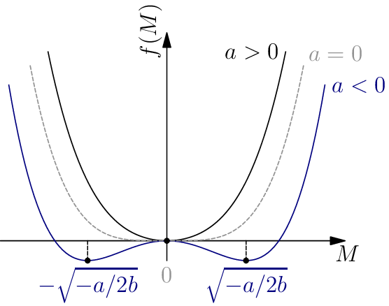
Therefore, the transition temperature $T_c$ corresponds to the zero of the function $a(T)$; the analyticity of $F$ means that we can expand it in a series,

$$ a(T)=A \, (T-T_c) + O(|T-T_c|^2) ,\;\Rightarrow\; a<0,\;\text{for } T<T_c $$

such that $a(T_c)=0$, with $A$ a constant. Replacing this expression into the equilibrium magnetization, we obtain

$$ M \sim |T-T_c|^\beta,\quad \beta = 1/2\,, $$

with the same exponent as the one obtained in mean field approximation of the ising model.

The homogeneous state is not structurally stable near the transition: spatial fluctuations become dominant in the limit $T\rightarrow T_c$. The physical manifestation of that is the presence of divergences in the response coefficients, like the susceptibility (a scalar in an isotropic medium, but more generally a tensor when it relates vectors):

$$ \begin{align*} \bm M(\bm x) &= -\frac{\delta F}{\delta \bm H(\bm x)},\\ \chi_{ij}(|\bm x - \bm x'|) &= \frac{\delta M(\bm x)}{\delta H(\bm x')} = -\frac{\delta^2 F}{\delta H_i(\bm x) \delta H_j(\bm x')}, \end{align*} $$

(where $H_i$ is one vector component of $\bm H$) computed at equilibrium, where the system is statistically translation invariant (the susceptibility only depends on the distance between two points).

Near thermodynamic equilibrium a universal relation exists between the linear response susceptibility $\chi$ and the correlation function $C$

$$ C_{ij}(|\bm x-\bm x'|) = \langle M_i(\bm x) M_j(\bm x') \rangle - \langle M_i(\bm x)\rangle \langle M_j(\bm x)\rangle\,, $$

of the corresponding physical quantity. Indeed, using the partition function in the form,

$$ Z(T, H)=\int D[\bm M]\, \E^{-F[\bm M]/ T - \int \D \bm x\, \bm H \cdot \bm M/T} $$

one can compute the second functional derivatives with respect to any vector coordinate,

$$ \chi=\frac{\delta F}{\delta H \delta H'}= T \left[ \frac{1}{Z} \frac{\delta^2 Z}{\delta H \delta H'} - \frac{1}{Z} \frac{\delta Z}{\delta H} \frac{1}{Z} \frac{\delta Z}{\delta H'} \right] = \frac{1}{T} \left[\braket{MM'}-\braket{M} \braket{M'} \right] $$

we obtain, at $H=0$, the fluctuation-dissipation theorem

$$ C_{ij}(|\bm x - \bm x'|) = T \chi_{ij}(|\bm x - \bm x'|)\,. $$

In the equilibrium state the magnetization has a constant value $M = \bar{m}$, different in each phase, $\bar{m}=0$ (paramagnetic state), and $\bar{m}=[A(T_c-T)/2b]^{1/2}$ (ferromagnetic state); around this equilibrium state, the order parameter fluctuates,

$$ \bm M(\bm x) = [\bar{m} + \phi_0(\bm x) ] \bm n + \bm \phi_\perp(\bm x) $$

where we defined the fluctuation field $\bm \phi$, which is decomposed into a longitudinal direction $\hat{\bm n}$ (the direction of the applied field) of amplitude $\phi_0$, and a transverse one $\bm \phi_\perp$.

Substituting this expansion into the free energy one gets $F=F[\bar{m}] + F[\phi_0] + F[\bm\phi_\perp]$,

$$ F[\phi_0] = \int \D \bm x \, [ \tfrac{\kappa}{2} (\nabla \phi_0 )^2 + (a+6b \bar{m}^2) \phi_0^2 ] $$

and

$$ F[\bm\phi_\perp] = \int \D \bm x \, [ \tfrac{\kappa}{2} |\nabla \bm\phi_\perp |^2 + (a+2b \bar{m}^2) \phi_\perp^2 ] $$

to lowest order in the fluctuating fields. The coefficients of the quadratic terms are related with the correlation lengths

$$ \frac{\kappa}{\xi_{0,\perp}^2} \equiv \left.\frac{\partial^2 f}{\partial \phi_{0,\perp}^2}\right|_{\bar{m}} \,. $$

Explicit computation gives the correlations lengths for the longitudinal,

$$ \kappa/2\xi_0^2 = a + 6 b \bar{m}^2 = \{A(T-T_c), \text{ if } T>T_c\,;\; 2A(T_c-T), \text{ if } T<T_c\}\,, $$

and the transverse fluctuations:

$$ \kappa/2\xi_\perp^2 = a + 2 b \bar{m}^2 = \{A(T-T_c), \text{ if } T>T_c\,;\; 0, \text{ if } T<T_c \}\,. $$

In analogy with the harmonic oscillator, this term is a restoring force; and it is zero for the transverse fluctuations in the ordered state: the correlation length goes to infinity. Fluctuations in the transverse direction give rise to oscillations of the magnetization around its mean direction, magnetization waves (Goldstone modes of low energy, arising from the breaking of a continuous symmetry, rotation here).

The bilinear free energy in the fluctuating fields $\phi_\alpha$ ($\alpha=0,\perp$), can be written as,

$$ F[\phi_\alpha] = \int \frac{\D \bm q }{(2\pi)^3} \frac{\kappa}{2\xi_\alpha^2} \big[ 1+(\xi_\alpha q)^2 \big] \phi_\alpha(\bm q) \phi_\alpha(-\bm q) $$

in Fourier space, where $\xi_\alpha = \xi_0, \xi_\perp$ for the two modes.

The correlation function can be found using the fluctuation-dissipation theorem. We add and external field term $\bm h$,

$$ F[\phi_\alpha,h_\alpha] = F[\phi_\alpha] - \int \frac{\D \bm q }{(2\pi)^3} h_\alpha(\bm q) \phi_\alpha(-\bm q) $$

and compute first the susceptibility using its definition

$$ \chi_\alpha(\bm q) \delta_{\bm q, \bm q'}= \frac{\delta \braket{\phi_\alpha}(\bm q) }{\delta h_\alpha(\bm q')}, $$

and the equilibrium condition,

$$ 0 = \frac{\delta }{\delta h_\alpha(\bm q)} \left( \frac{\delta }{\delta \phi_\alpha(-\bm q')} F[\phi_\alpha, h_\alpha] \right) $$

The first functional derivative gives,

$$ \frac{\delta }{\delta \phi_\alpha(-\bm q')} F[\phi_\alpha, h_\alpha] = \frac{\kappa}{\xi_\alpha^2} \big[ 1+(\xi_\alpha q')^2 \big] \braket{\phi_\alpha}(\bm q') - h_\alpha(\bm q') $$

and the functional derivative of this expression with respect to the field, yields

$$ 0 = \frac{\kappa}{\xi_\alpha^2} \big[ 1+(\xi_\alpha q)^2 \big] \chi_\alpha(\bm q)\delta_{\bm q, -\bm q'} - \delta_{\bm q, -\bm q'} $$

(note the factor 2) where we replaced the functional derivative of the fluctuation with respect to the field by the susceptibility.

One finally obtains the susceptibility

$$ \chi_\alpha(\bm q) = \frac{1}{\kappa} \frac{\xi_\alpha^2}{1 + (\xi_\alpha q)^2} $$

and, form the fluctuation-dissipation relation, the structure function,

$$ S_\alpha(\bm q) = \braket{\phi_\alpha(\bm q) \phi_\alpha(-\bm q)} = \frac{T}{\kappa}\frac{\xi_\alpha^2}{1 + (\xi_\alpha q)^2} $$

The structure function (in the mean field theory) in the ferromagnetic state. The longitudinal fluctuations $S_l$ have a lorentzian spectrum; the transverse fluctuations diverge at large wavelengths. At the critical temperature both spectra diverge as $\sim 1/q^2$ for $q \rightarrow 0$.

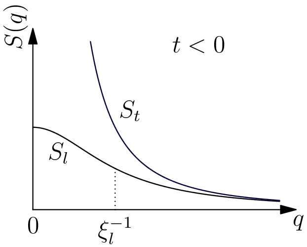
At the critical temperature both susceptibilities diverge $\chi_\alpha \sim 1/q^2$, or in real space $\chi_\alpha(r) \sim 1/r$ EX, but the perpendicular one is divergent in the whole ordered phase. The longitudinal susceptibility represents the response of the magnitude of the order parameter, while the perpendicular one describes the response to a change in direction of the magnetization: in the ordered phase changing the direction of all spins (rotating the perpendicular vector around the longitudinal one), do not cost much energy: the perpendicular mode is called the soft mode, and extending it to the frequency domain (time dependent fluctuations) shows the presence of “spin” waves. This phenomenon is general to the breaking of a continuous symmetry (rotation).