\(\newcommand{\I}{\mathrm{i}} \newcommand{\E}{\mathrm{e}} \newcommand{\D}{\mathop{}\!\mathrm{d}} \newcommand{\bra}[1]{\langle{#1}|} \newcommand{\ket}[1]{|{#1}\rangle} \newcommand{\braket}[1]{\langle{#1}\rangle} \newcommand{bm}{\boldsymbol}\)
Workshop on scientific typesetting.
Scientific writing with \(\LaTeX\)
The goal of this course is to learn how to use the tools allowing to write scientific documents of high quality. The \(\LaTeX\) typesetting system is universally used in the scientific and technical literature; it is based on the language \(\TeX\) created by Donald Knuth.
You will write a short article using your own lecture notes from one of the license or master courses you attended. Typically, you take a simple subject, like the pendulum, the Carnot cycle, or the electric field of a dipole, and write a self-contained text in the form of a scientific paper. Your document should comply with the standards of the scientific papers: front matter, abstract, introduction, main content, conclusion, and references.
A reasonable, minimal, scientific computing environment might consist in:
- A \(\LaTeX\) distribution (TeXLive, see the references at the end of this page, is the standard one)
- An editor: TeXMaker, vim, or equivalent
- A
pythonprogramming environment (you may use Anaconda)
(preferably in a unix-like system!).
LaTeX language
A LaTeX document is written in plain text using an editor like “vim”. The file name extension is .tex. Once compiled, it produces an output file, generally in the .pdf format:
$> pdflatex filename.tex
where $> is the unix shell prompt and pdflatex the TeX compilation command. Instead, you may also use lualatex command if you want for instance, write your text with the system’s fonts or implement modern language features. If the compilation stops in an error, you may recover your session using crtl-D. In practice, the compilation of the source file .tex can be done directly from the text editor, without the need of a terminal.
The complex compilation process, for documents containing table of contents, tikz or asymptote graphs and bibliography, for example, can be automated using the latexmk tool.
The LaTeX source files start with a \documentclass[options]{class} command. Every tex command starts with a backslash \, and may contain options (within square brackets []) and arguments (within curly brackets {}). The head of the source file is called the preamble, and contains a series of commands to load the LaTeX packages (utility libraries). The body of the document is written in the document environment:
\documentclass[opt]{arg}
.
.
.
\begin{document}
.
.
.
\end{document}
An environment has the structure \begin{cmd}...\end{cmd}, and is used for equations, lists, figures, etc.
The title, author and date are filled in the preamble, and generated by \maketitle, just after the beginning document environment.
The text is structured in sections \section{Title} (chapters for a book), subsections, etc.; paragraphs are separated by a blank line. Spaces and tabs are treated as single spaces. A single “line break” (return or enter) does not change the line; to change the line (within the same paragraph, for example in a poem) you may use a double backslash \\. Comments are lines starting with a percentage %. The reserved language characters are:
# $ % ^ & _ { } ~ \
to write these symbols in your text you prepend them with a backslash (e.g. \%).
List environments are itemize, enumerate and description. Mathematics is written inline using single dollars $...$, or preferably \(...\), and displayed (in their own line) using double dollars $$...$$, or preferably \[...\]; equation environments (with label and number)
are equation, align, etc.:
\begin{equation}
\label{eq}
....
\end{equation}
Reference to the equation, in this example, is made by \ref{eq}.
Tables are typeset with the tabular environment; each item is separated by &; each line is terminated be \\:
\begin{tabular}[htb]{columns spec}
\hline
... & ... \\
\haline
...
\end{tabular}
Tabular is a floating environment, its position in the page depends on the context. Another floating is figure:
\begin{figure}[htb]
  \centering
  \includegraphics[width=0.8\textwidth]{fig_name}
  \caption{fig_name has extension pdf, png or jpg; options include width, height, scale, etc.
    \label{f:your_label}}
\end{figure}
used to insert a figure, the command \includegraphics belong to the graphicx package.
To emphasize text use \emph{...}; \textbf{...} is bold text.
Typesetting mathematics is straightforward:
- Inline formula
\(...\), displayed\[...\] - Equation with number
\begin{equation}...\end{equation} - Sequence of centered formulas
\begin{gather}...\end{gather}, aligned at&,\begin{align}...\end{align} - Raw formulas
a+b=c: \(a+b=c\) - Sub and superscripts
_and^,a_2x^2+a_1x+a_0=0: \(a_2x^2+a_1x+a_0=0\) (spaces are not significant in math formulas) - Fractions
\frac{a}{b+c}:$$\frac{a}{b+c}$$ - Integrals and sums
\int_0^1 dx f(x) = 1,\sum_{n=0}^\infty \frac{x^n}{n!}= \mathrm{e}^x\begin{gather*} \int_0^1 dx f(x) = 1 \\ \sum_{n=0}^\infty \frac{x^n}{n!}= \mathrm{e}^x \end{gather*} - Limits
\lim_{x \rightarrow 0} \frac{\sin x}{x} = 1$$\lim_{x \rightarrow 0} \frac{\sin x}{x} = 1$$ - Greek letters
\alpha, \beta, \gamma, \ldots: \(\alpha, \beta, \gamma, \ldots\) - roman, blackboard and calligraphic symbols
\mathrm{i},\mathbb{R},\mathcal{L}: \(\mathrm{i},\mathbb{R},\mathcal{L}\) - Vectors (bold mathematics
\usepackage{bm}),\bm{a = b \times c}\(\bm{a = b \times c}\) - Square root
\sqrt{1+ \mathrm{i}}: \(\sqrt{1+\mathrm{i}}\) - Large parenthesis
\left(1+\frac{x}{n}\right)^n \rightarrow \mathrm{e}^{-x}:$$\left(1-\frac{x}{n}\right)^n \rightarrow \mathrm{e}^{-x}$$
LaTeX template
Important advice: do not try by any means to format your text, use exclusively the latex environments for your layout. Avoid \\, vspace, clearpage; do not modify the margin sizes (the use of the geometry package must not break the basic typographic rules).
Define the document class: article, report, book, standalone, etc.
\documentclass[a4paper, 11pt, twoside]{article}
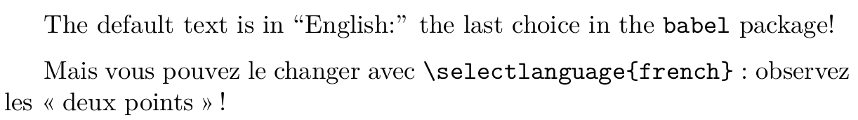
Define the text encoding as utf8, and fonts: lmodern, latin modern is the standard font, based on the famous “Computer Modern” font designed by Donald Knuth. You may choose other fonts (see the \(\LaTeX\) fonts catalogue); a modern complete set of font is STIX. The package babel defines specific language typesetting; the last one in the list (here english) is the active one. To activate french use the command \selectlanguage{french}. You may toggle between languages using \selectlanguage.
%
% fonts and languages
    \usepackage[utf8]{inputenc}
    \usepackage[T1]{fontenc}
    \usepackage{lmodern}
    \usepackage[french,english]{babel}
%
The first part of the source document, after the documentclass declaration, is the “preamble”; the text body is written inside the document environment:
\begin{document}
  The default text is in ``English:'' the last choice in
  the \texttt{babel} package!

  \selectlanguage{french}
  Mais vous pouvez le changer avec \verb+selectlanguage{french}+:
  observez les \og deux points \fg!
\end{document}
The preamble contains the list of packages, tex libraries necessary to type complex mathematics, insert figures, or customize the text layout, the bibliography, etc.:
%
% AMS math
    \usepackage{amsmath}
    \usepackage{amssymb}
    \usepackage{bm}
These packages define a large set of mathematical constructions, like the align, gather or multiline environments, and adds special symbols (\(\mathfrak{H}\)) and bold mathematics (\bm y: \(\boldsymbol y\)):
  Maxwell equations,
  \begin{gather}
    \label{e:ME}
    \nabla \cdot \bm E = \frac{\rho}{\epsilon_0}\,, \\
    \nabla \times E = -\frac{\partial \bm B}{\partial t} \\
    \nabla \cdot \bm B = 0 \\
    \nabla \times \bm B = \mu_0 \bm j -
               \mu_0\epsilon_0 \frac{\partial \bm E}{\partial t}
  \end{gather}
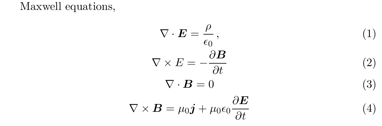
Equation numbers can be referred using \eqref{label} (ams package).
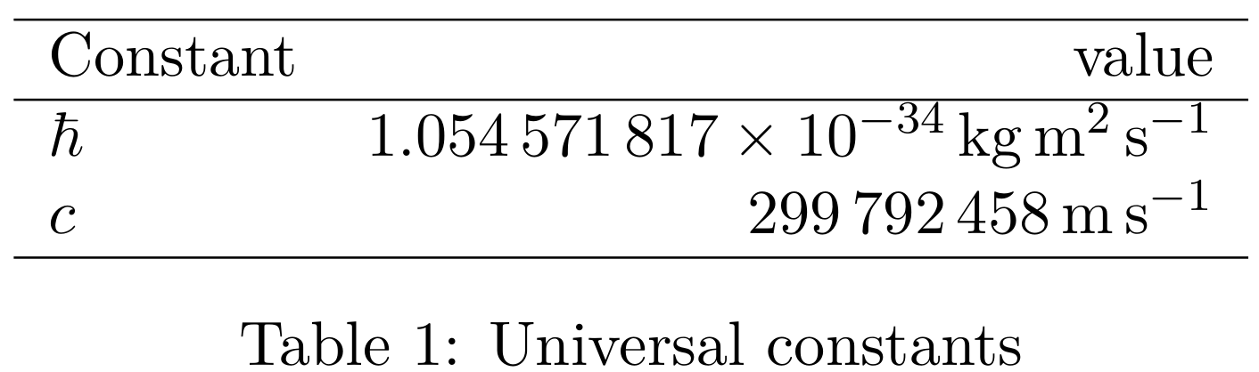
The package siunitx setup numbers and units (SI system):
  \usepackage{siunitx}
  .
  .
  .
  \begin{table}[h]
  \centering
  \begin{tabular}{lr}
    \hline
    Constant & value \\
    \hline
    $\hbar$ & \SI{1.054571817E-34}{\kilogram \square\meter \per \second}\\
    $c$     & \SI{299 792 458}{\meter \per \second}\\
    \hline
\end{tabular}
\caption{Universal constants}
\label{t:h}
\end{table}
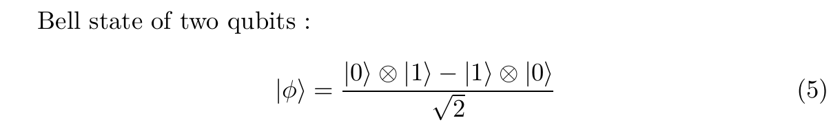
Utility packages, as the small braket one, helps to specific needs:
  \usepackage{braket}
  .
  .
  .
  Bell state of two qubits:
  \begin{equation}
    \label{e:q}
    \ket{\phi} = \frac{\ket{0} \otimes \ket{1} -
                       \ket{1} \otimes \ket{0}}{\sqrt{2}}
  \end{equation}
Figures are loaded with the graphicx package; hyperlinks are managed by hyperref; coloring text and boxes is done with xcolor:
%
% Graphics
    \usepackage{graphicx}
    \usepackage[x11names,table]{xcolor}
%
% References and links
    \usepackage{url}
    \usepackage{doi}
    \usepackage{hyperref}
    \hypersetup{colorlinks,%
      linkcolor=SkyBlue4,%
      urlcolor=Blue4,%
      citecolor=Red4,%
      filecolor=Green4}
Aliases to often used commands can be defined with \newcommand:
%
% New commands
% language
    \newcommand{\FRA}{%
    \selectlanguage{french}}
    \newcommand{\ENG}{%
        \selectlanguage{english}}
% math
    \newcommand{\I}{\mathrm{i}}
    \newcommand{\E}{\mathrm{e}}
    \newcommand*{\D}{\mathop{}\!\mathrm{d}}
% constants
    \newcommand{\kB}{k_\textsc{b}}
    \newcommand{\NA}{N_\textsc{a}}
The following code inserts a floating figure:
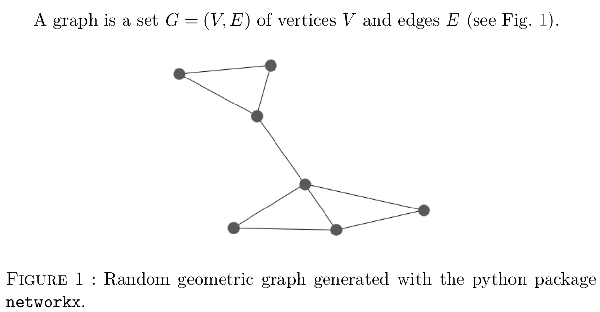
A graph is a set \(G = (V,E)\) of vertices \(V\) and edges
\(E\) (see Fig.~\ref{f:grg}).

\begin{figure}[h]
  \centering
  \includegraphics[width=0.49\textwidth]{grg.png}
  \caption{Random geometric graph generated with the python
  package \texttt{networkx}.
  \label{f:grg}}
\end{figure}
References
Installation
- In Linux install TeX Live over the internet: download the TeX Live installer, untar it
tar xvf install-tl-unx.tar.gz, change directory and run the perl script:cd install-tl-20191109and./install-tl; you may also need to update your path variableexport PATH=/usr/local/texlive/2019/bin/x86_64-linux:$PATH - For MacOs install MacTex
- For Windows install MikTeX. Use the net installer (instead of the basic one) to get a full distribution (Net Installer, CAUTION this is an executable file). Remark: you should launch the installer twice: first you download all packages, then you install the packages using the same Installer 64-bit! (instructions en français: https://www.xm1math.net/doculatex/install_miktex.html)
- To manage efficiently the bibliography you may use Zotero with the bibtex plugin Better Bibtex and the files plugin ZotFile.
- Installing python is easy with Anaconda: choose the installer for your system.
Documentation
- Full archive of latex resources CTAN
- A not so short introduction to \(\LaTeX\), by by Tobias Oetiker.
- Short guide to typset mathematics, by Michael Downes, updated by Barbara Beeton.
- Exposé sur \(\LaTeX\), par Thierry Masson.
- Wikibook LaTeX, highly recommended.