\(\newcommand{\I}{\mathrm{i}} \newcommand{\E}{\mathrm{e}} \newcommand{\D}{\mathop{}\!\mathrm{d}} \newcommand{\bra}[1]{\langle{#1}|} \newcommand{\ket}[1]{|{#1}\rangle} \newcommand{\braket}[1]{\langle{#1}\rangle}\)
Workshop on scientific typesetting.
Document structure
The .tex source file start with the \documentclass command, followed by the preamble. The preamble contains the list of packages, definitions and new commands. A simple template to compiled with lualatex —shell-escape:
\documentclass[11pt,twoside]{article}
% luatex set fonts
    \usepackage{fontspec}
    \usepackage[bold-style=ISO]{unicode-math}
    \setmainfont{Latin Modern Roman}
    \setmathfont{Latin Modern Math}
%
% languages
    \usepackage{polyglossia}
    \setdefaultlanguage[variant=american]{english}
    \setotherlanguage{french}
%
% math
    \usepackage{lualatex-math}
    \usepackage{mathtools}
    \usepackage{siunitx}
%
% Graphics
    \usepackage{tikz}
    \usepackage{graphicx}
%
\begin{document}
%
your text
%
\end{document}
You may add your own packages:
%
% References and links
    \usepackage{url}
    \usepackage{hyperref}
    \hypersetup{colorlinks,%
      linkcolor=blue!80!green!70!red,
      urlcolor=blue!50!black,
      citecolor=red!50!black,
      filecolor=green!50!black}
%
% Tables, code and lists
    \usepackage{minted}
    \setminted{fontsize=\footnotesize}
    %
    \usepackage{booktabs}
and definitions:
    %
    \DeclarePairedDelimiter\bra{\langle}{\rvert}
    \DeclarePairedDelimiter\ket{\lvert}{\rangle}
    \DeclarePairedDelimiter\braket{\langle}{\rangle}
    \DeclarePairedDelimiter\List{\{}{\}}
    \DeclarePairedDelimiterX\Inner[2]{\langle}{\rangle}%
      {#1 \delimsize\vert \mathopen{}#2}
    \DeclarePairedDelimiterX\Mean[3]{\langle}{\rangle}%
      {#1\,\delimsize\vert\,\mathopen{}#2\,\delimsize\vert\,\mathopen{}#3}
    \newcommand{\bm}{\symbf}
    \newcommand{\I}{\symup{i}}
    \newcommand{\E}{\symup{e}}
    \newcommand*{\D}{\mathop{}\!\symup{d}}
Lualatex is a modern alternative to pdflatex.
The text of your document may contain:
- the top matter: title, author, institution, address, date; this information can be put in the preamble and typeset with
\maketitle:
\title{Vectorial Space Structure of the Set of Cycles of a Graph}
\author{Marc Dupont\\
        Département de physique, Université d'Aix-Marseille, France}
\date{November, 2020}
\begin{document}
\maketitle
\end{document}
-
an abstract: short description of the article, underlying the problem addressed and the main result
-
An introduction: general description of the subject and its scientific context; citation to the previous works; statement of the problem and the approach to deal with it, rough description of the model; summary of the article contents.
- The model, experimental setup or numerical and analytical methods, results and discussion, are presented in separated sections and constitute the main contents of the article.
- The article is closed with a generally brief conclusion.
- The end matter may contain appendices to the main text, and the references to the cited literature.
In order to structure your text you may use the \section and \subsection commands:
\documentclass[]{article}
...
\title{...}
\author{...}
\date{...}
\begin{document}
\maketitle

\begin{abstract}
...
\end{abstract}

\tableofcontents % automatically creates a table of contents
                 % based on the structure in sections of the article

\section{Introduction}
Scientific context, motivation, references, statement of
the problem and paper structure.

\section{Model}
...

\section{Results}
...

\subsection{Case A}
...

\subsection{Case B}
...

\subsubsection{Case BA}
...

\section{Conclusion}
Short description of the model and results, discussion of
open issues and outlook.

\printbibliography % with biblatex
\end{document}
The bibliography
Bibtex is the bibliography database management program for latex documents. You create a .bib bibliographic data base in the bibtex format. It is convenient to use the biblatex package and the biber engine:
    \usepackage[
      backend=biber,
      style=numeric,
      firstinits=true,
      natbib=true,
      sorting=none,
      url=false,
      doi=true,
      eprint=true
      ]{biblatex}
    \bibliography{bibfile}
you put in the preamble, where bibfile is the name of your database tplatex.bib, in the example. Then, you put the command \printbibliography where you want the bibliography, in general just before the end of the document.
An article entry of a .bib file looks as:
@article{Schrodinger-1935,
  title = {Discussion of Probability Relations
           between Separated Systems},
  author = {Schrödinger, E.},
  journal = {Mathematical Proceedings of the
             Cambridge Philosophical Society},
  volume = {31},
  number = {4},
  pages = {555-563},
  year = {1935},
  doi = {10.1017/S0305004100013554}
}
or a more recent one, with and url field in addition to the doi one:
@article{Georgescu-2014,
  title = {Quantum Simulation},
  author = {Georgescu, I. M. and Ashhab, S. and Nori, Franco},
  journal = {Rev. Mod. Phys.},
  volume = {86},
  number = {1},
  pages = {153-185},
  year = {2014},
  doi = {10.1103/RevModPhys.86.153},
  url = {https://link.aps.org/doi/10.1103/RevModPhys.86.153}
}
A book entry:
@book{Wen-2004,
  title = {Quantum Field Theory of Many-Body Systems:
           From the Origin of Sound to an
           Origin of Light and Electrons},
  shorttitle = {Quantum Field Theory of Many-Body Systems},
  publisher = {{Oxford University Press on Demand}},
  author = {Wen, Xiao-Gang},
  year = {2004}
}
To compile a document containing a \bibliography you must execute the sequence:
> pdflatex yourtexfile.tex
> bibtex yourtexfile   # or "biber" if you use biblatex
> pdflatex yourtexfile.tex
> pdflatex yourtexfile.tex
Three pdflatex compilations and one bibtex compilation are necessary.
To create your bibliographic database you may find it useful to install Zotero, as suggested in the previous lecture.
Example
The following snippets illustrate the standard structure of a research paper. We start with the abstract.
\begin{abstract}
We investigate the structure of the cycle space of a graph and show that it is
possible to assign to it a vector space over $GF(2)$, with the symmetric difference
as the composition rule.
\end{abstract}
The first section is the introduction.
\section{Introduction}

In 1935 Schrödinger defined entanglement as the distinctive
property of quantum mechanics \cite{Schrodinger-1935}.
It is interesting to note that, in addition to the usual
definition in terms of the separability of a composite
system state (the ``representative'' in his words) into a
product of individual factors corresponding to each
constituent, he put forward the fact that the information
contained in the whole cannot be necessarily obtained from
the information contained in its parts, implicitly
expressing that entanglement is an information resource.
Since then the double status of the quantum state as
physical and informational has gained in importance to
characterize a great variety of phenomena
\cite{Stanescu-2016,Zeng-2019}, ranging from quantum computing
\cite{Nielsen-2010fk,Georgescu-2014} to topological phases
in condensed matter \cite{Fradkin-2013,Wen-2017}.
The main part of the article describes the model, results and discussion.
\section{Model}
A cycle \(b\) is a closed path in \(G\); it is a subset
of the graph edge set \(E\). The set \(B_C(G)\) of all
cycles is the cycle space. To each cycle \(b \in B_C(G)\)
we can associate a vector with \(|E|\) components, each
taking the values in the set \(\{0,1\}\), where the value
\(1\) stands for an edge in \(b\), and \(0\) otherwise.
The cycle space \(B_C(G)\) equipped with the ring sum
forms a vector space over the finite field \(\mathrm{GF}(2)\),
of dimension \cite{Gross-2005},
\begin{equation}
  \label{e:dimB}
  |B| = |E| - |V| + 1
\end{equation}
(for a connected graph). The composition rule of the vector
space, the ring sum \(b_1 \oplus b_2\), corresponds to the
symmetric difference between the edges subsets
\((b_1 \cup b_2) \setminus (b_1 \cap b_2)\). A set of cycles
that cannot be written one another as a ring sum combination,
is an independent set. A set \(B \subset B_C\) of independent
cycles of dimension \(|B|\), given by \eqref{e:dimB}, is a
cycle basis \(B\):
\begin{equation}
  \label{e:setB}
  B = \{b_n \in B_C,\; n=1,\ldots,|B|\}\,,
\end{equation}
of \(B_C\). Therefore, every element \(b\in B_C\) can be
written as a linear combination of the basis cycles:
\[b = \sum_{n = 1}^{|B|} s_n b_n,\quad s_n = 0, 1\,.\]
We call the minimum cycle basis of \(B_C\), the basis of
shortest length \cite{Kavitha-2009},
\begin{equation}
  \label{e:Bmin}
  B_G = \left\{ b_n \in B \,|\, \min \len(B) \right\}
\end{equation}
where,
\[\len(B) = \sum_{n=1}^{|B|} \len(b_n) \]
with the length of a cycle \(b\) defined as the total number
of its nodes:
\[\len(b) = |b|\,.\]
One ends with the conclusion and outlook.
%
\section{Conclusions}
%

Using a model of an interacting quantum system introduced
in \cite{Verga-2019}, we investigated the entanglement
structure of the thermal state. The model do not contain
dimensional parameters: it is essentially defined by the
graph\ldots
Collecting all the code snippets you get a pdf like the one in this link.
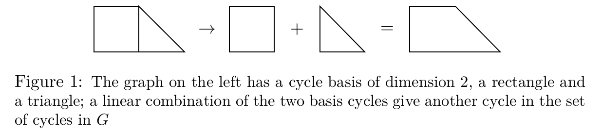
The general presentation should be simple and clear, the essential questions and achievements of the work well identified. For instance, to better explain the concept of cycle basis it is convenient to draw a graphical example:
\newcommand{\Rc}{\draw (0,0)--(0,1)--(1,1)--(1,0)--cycle}
\newcommand{\Tc}{\draw (1,0)--(1,1)--(2,0)--cycle}
\begin{figure}[hb]
  \centering
\begin{tikzpicture}
  \Rc;
  \Tc;
  \node at (2.5,0.5) {$\rightarrow$};
  \begin{scope}[shift={(3,0)}]
    \Rc;
    \node at (1.5,0.5) {$+$};
    \begin{scope}[shift={(1,0)}]
      \Tc;
      \node at (2.5,0.5) {$=$};
    \end{scope}
    \begin{scope}[shift={(4,0)}]
      \draw (0,0)--(0,1)--(1,1)--(2,0)--cycle;
    \end{scope}
  \end{scope}
\end{tikzpicture}
\caption{\small The graph on the left has a cycle basis of
dimension 2, a rectangle and a triangle; a linear
combination of the two basis cycles give another cycle
in the set of cycles in $G$}
\end{figure}
How to make graphics like this one is the subject of the next lecture.
References
-
Interesting article about luatex by Lee Phillips.
-
The text fragments are form a paper by Verga and Elías, 2019
-
Writing scientific papers: the guidelines to authors of SciPost and the APS author guidlines are representative of the publishing scientific research process.