$\newcommand{\I}{\mathrm{i}} \newcommand{\E}{\mathrm{e}} \newcommand{\D}{\mathop{}\!\mathrm{d}} \newcommand{\Di}[1]{\mathop{}\!\mathrm{d}#1\,} \newcommand{\Dd}[1]{\frac{\mathop{}\!\mathrm{d}}{\mathop{}\!\mathrm{d}#1}} \newcommand{\bra}[1]{\langle{#1}|} \newcommand{\ket}[1]{|{#1}\rangle} \newcommand{\braket}[1]{\langle{#1}\rangle}$

»quantum chaos »kicked rotator »random matrices »quantum walk

Dynamical localization

Anderson (1958) discovered that disorder leads to localization of the quantum states. Contrary to naive physical “intuition”, transport in a metal with a strong concentration of impurities do not proceed by tunneling from one impurity to another, but completely stops above a threshold concentration: if initially the particle probability is concentrated at the origin, the probability of finding the particle at the origin when times goes to infinity, remains finite. Therefore the particle’s wave function is exponentially localized inside a region characterized by a localization length $l$.

A simple model of localization consists in a tight-binding one dimensional Hamiltonian $H$ with random energies $\varepsilon_x$ at each lattice site $x$ (we take the lattice step $a=1$ as the unit of length), and a constant hopping energy between neighboring sites (taken to be the unit of energy and $\hbar=1$):

\begin{equation} H = -\sum_x \left( |x+1\rangle \langle x| + |x-1\rangle \langle x| \right) + \sum_x \varepsilon_x |x\rangle \langle x| \,, \label{alH} \end{equation}

where $\varepsilon_x \sim \mathcal{U}(-W/2,W/2)$ are uniformly distributed in a band of width $W$, and $|n\rangle$ is the position state. The first term of $H$ contains the random energies, and the two last terms the hopping energies to the right or to the left of point $x$. This model, proposed by Anderson, exhibit in one and two dimensions, complete localization for any disorder strength (measured by $W$), and in three dimensions for disorder strengths above a threshold.

The solution of the stationary Schrödinger equation,

\begin{equation} H |E_n\rangle = E_n |E_n \rangle\,, \quad n = 0,1,\ldots \label{alEV} \end{equation}

are the energy eigenvectors $\langle x|E_n\rangle = \psi_n(x)$ and $E_n$ the corresponding eigenvalues. This eigenvalue problem can easily be solved numerically.

Exercice

Compute the eigenvectors and eigenvalues of the Anderson Hamiltonian ($\ref{alH}$), and show in particular that the histogram of energy level spacings $s=(E_{n+1} - E_n)/\overline{\Delta E}$ follows a Poisson law.

from numpy.random import random, uniform
from numpy.linalg import eig, eigvals
def hamiltonian(L = 1024, W = 2.0):
    return -roll(eye(L), -1) - roll(eye(L), +1) + diag(uniform(-W/2, W/2, L))

L = 1250
W = 2.0
H = hamiltonian(L = L, W = W)
E, U = eig(H)
U = U[E.argsort()]
E.sort()

energy mode spacings

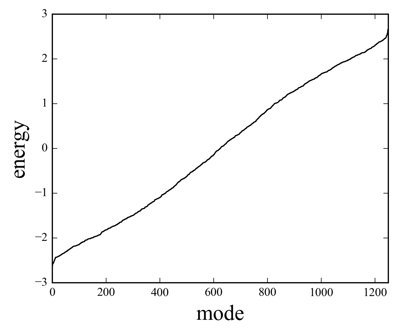
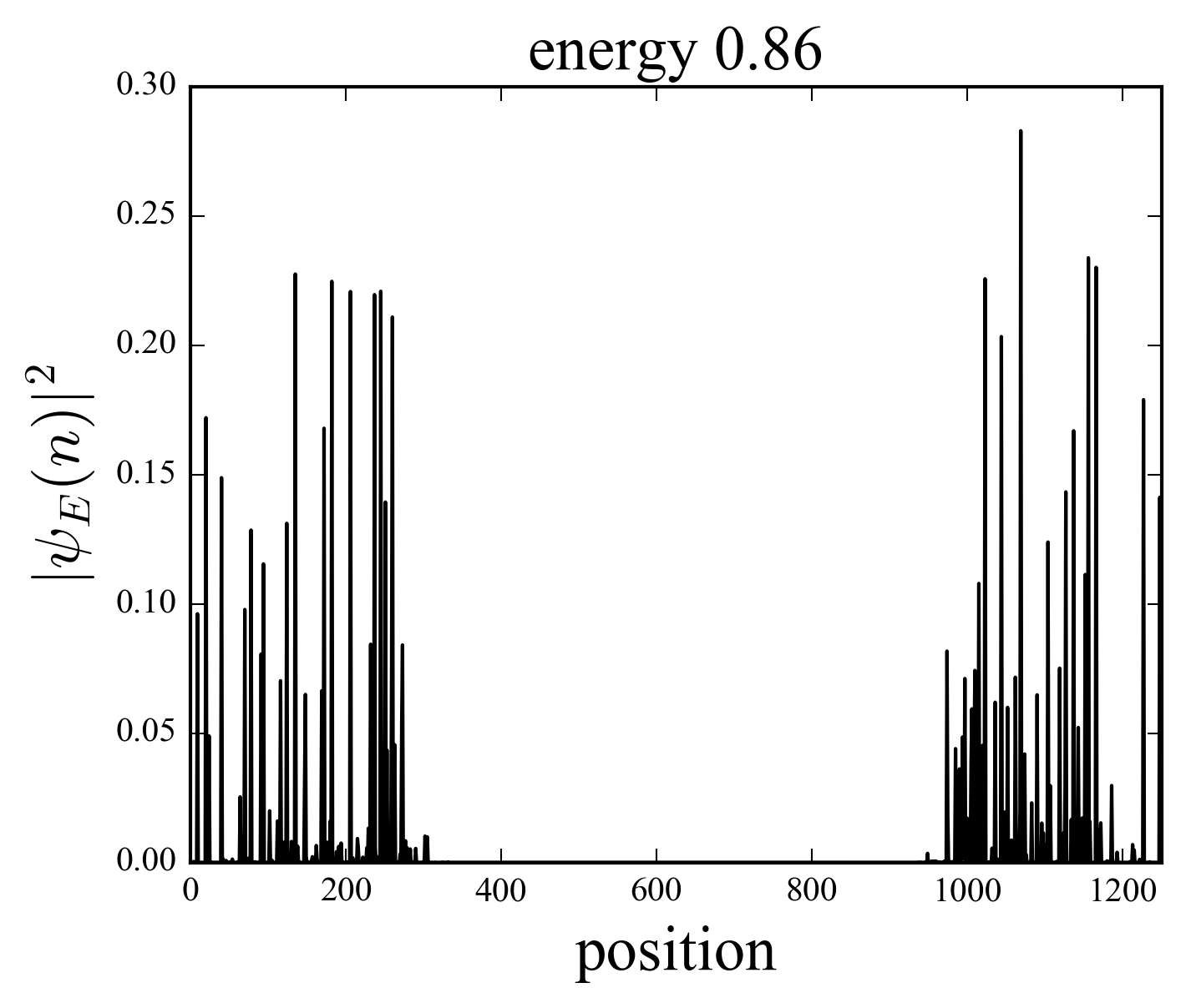
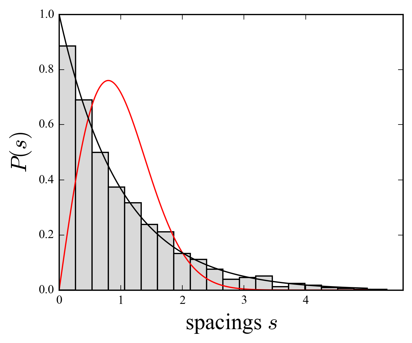
The above figures show the spectrum of the random Hamiltonian, a typical eigenvector (in one dimension all the eigenvectors are localized), and a histogram showing that the energy spacing follows a Poisson distribution. This distribution is different from the random matrix distribution of the Gaussian orthogonal ensemble (valid for real symmetric matrices whose entries are Gaussian random numbers), which characterizes time reversal symmetric Hamiltonians. The main difference between the matrix $H$ and the Gaussian matrix is that its diagonal terms are uncorrelated; the Gaussian matrix can be diagonalized, but its eigenvalues will have strong correlations.

The Schrödinger equation with energy $E$, can also be written as a second order difference equation

\begin{equation} \psi_{x+1} + \psi_{x-1} + (E - \varepsilon_x) \psi_x = 0\,, \label{alS} \end{equation}

where $\psi_x = \langle x | \psi \rangle$ is the particle wave function, the probability amplitude to find the particle at site $x$. This form is well adapted to investigate the transmission $T$ through a lattice of length $L$, as a function of the energy $E$, of an incident particle $\E^{\I kx}$ (plane wave), where $k$ is given by

$$E = -2 \cos(k)\,,$$

the dispersion relation of a free particle ($\varepsilon_x=0$), propagating from left to right. Equation ($\ref{alS}$), can be put in a more convenient form, using the matrix $M_n$,

\begin{equation} \begin{pmatrix} \psi_{x+1} \\ \psi_x \end{pmatrix} = M_x\,\begin{pmatrix} \psi_{x} \\ \psi_{x-1} \end{pmatrix}\,, \quad M_x = \begin{pmatrix} -(E-\varepsilon_x) & -1 \\ 1 & 0 \end{pmatrix}\,; \label{alM} \end{equation}

the matrix $M_x$ is unimodular ($\det M_x =1$). Therefore, the initial value problem of the Schrödinger equation is solved by the product of random matrices:

$$ \begin{pmatrix} \psi_{x+1} \\ \psi_x \end{pmatrix} = M_x M_{x-1}\ldots M_1 \begin{pmatrix} \psi_{1} \\ \psi_0 \end{pmatrix} $$

A theorem on random unimodular matrices products due to Furstenberg (1963), states that

\begin{equation} \lim_{x\rightarrow \infty} \frac{1}{x} \ln \mathrm{Tr}\, (M_x\ldots M_1 ) = \lambda>0\,, \label{alF} \end{equation}

where $\lambda$ is the maximum Lyapunov exponent. As a consequence of the exponential growth of the matrix product, the asymptotic behavior of the wave amplitude must be of the form:

$$ \lim_{x \rightarrow \infty} \psi_x \sim \E^{\pm x/\ell}\,, \quad \ell \sim 1/\lambda\,.$$

Indeed, for generic initial conditions $(\psi_0,\psi_1)$, the solutions of the Schrödinger equation will be a superposition of growing and decaying amplitudes, whose characteristic length scale is a function of the energy, $\ell=\ell(E)$. Only for special values of the energy, precisely the eigenvalues of ($\ref{alEV}$), will result in normalizable solutions, simultaneously decaying in both directions.

In summary, the spectrum of the Anderson Hamiltonian is a discrete spectrum of exponentially localized wave functions, whose characteristic localization length is given by the inverse of the Lyapunov exponent of the transfer matrix product.

It is worth noting that equation ($\ref{alS}$) is analogous to the dynamical equation of a kicked Hamiltonian system, where position steps are replaced by time steps between kicks. This analogy allows to investigate the localization of the quantum kicked rotator using the methods developed to the Anderson problem.

Exercice

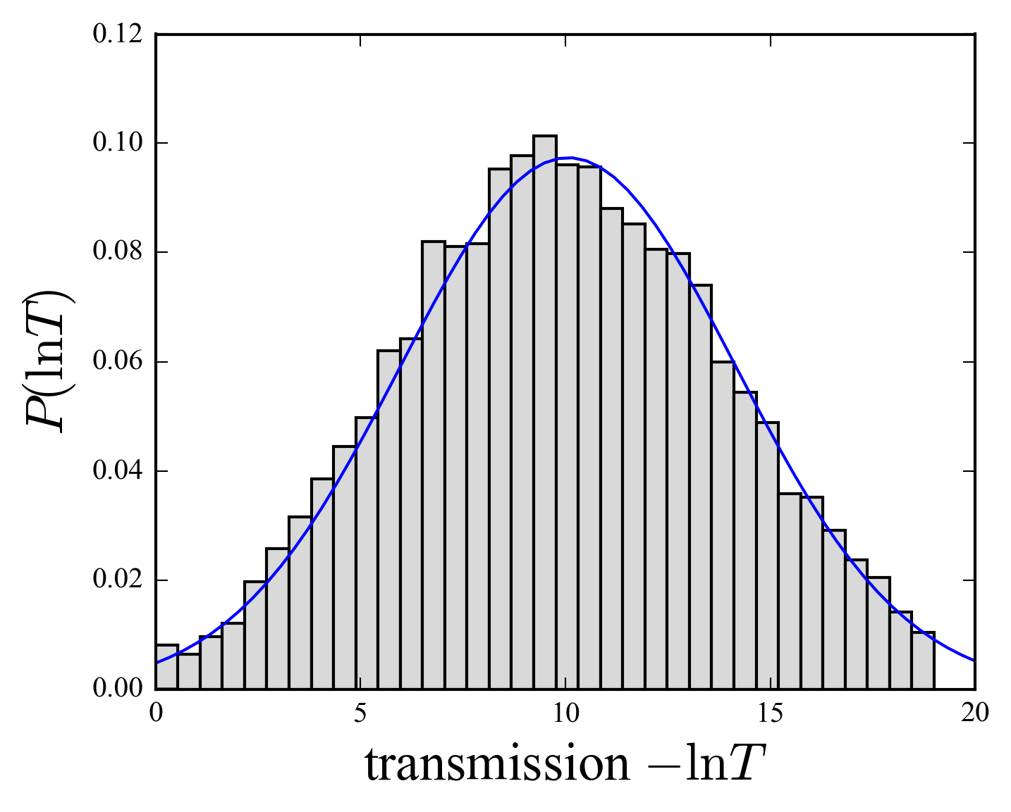
Compute the localization length and investigate the fluctuations of the transmission coefficient $T=T(E,L)$ of the one dimensional Anderson model. Solve ($\ref{alS}$) imposing an outgoing plane wave at site $L+1$: $\psi_{L+1}=\E^{\I k}$ and $\psi_L = 1$, and integrating the difference equation backwards in space. See the Markos (2006) paper, to find a computation of the transmission coefficient using the transfer matrix $T$
$$T_x = Q^{-1} M_x Q \,, \quad T^L = \begin{pmatrix} 1/t^* & -r^*/t^* \\ -r/t & 1/t \end{pmatrix} \,,\quad Q = \begin{pmatrix} 1 & 1 \\ \E^{-\I k} & \E^{\I k} \end{pmatrix}$$

amplitude transmission

# original perl code by Dominique Delande 
#   arXiv:1005.0915v2 (Les Houches, 2009)
#   http://arxiv.org/abs/1005.0915v2
#
def transmission(L = 1250, W = 0.6, E = 0.5, NA = 10000):
    #
    k = arccos(0.5*E)
    logT = zeros(NA)
    #
    # average over disorder
    for j in range(NA):
        #
        # initial plane wave (outgoing)
        psi_n_plus_1 = exp(1j*k)
        psi_n = 1.0
        e_n = W*(random(L) - 0.5)
        #
        # solve Schroedinger equation from last point
        for n in arange(L-1,0,-1):
            psi_n_minus_1 = (E - e_n[n])*psi_n - psi_n_plus_1
            (psi_n, psi_n_plus_1) = (psi_n_minus_1, psi_n)
        #
        # transmission coefficient $itt = 1/|t|^2$
        psi_n_minus_1 = E*psi_n - psi_n_plus_1
        itt = (0.5*abs(psi_n_minus_1 - exp(1j*k)*psi_n)/sin(k))**2
        logT[j] = log(itt)
        #
    return logT

Analogy of the kicked rotator with the Anderson model

A relation can be established between the Anderson model of spacial localization, and the dynamical localization in kicked systems. We start by using a Hermitian operator $W$ to transform the perturbation part of the Floquet operator $F=\E^{-\I V(x)} \E^{-\I H_0}$:

\begin{equation} \E^{-\I V(x)} = \frac{1 - \I W(x)}{1 + \I W(x)}\,, \quad W(x) = \tan \frac{V(x)}{2}\,. \label{alFW} \end{equation}

Substitution in the eigenvector formula $F |\phi\rangle = \E^{-\I \phi}|\phi\rangle$, gives

$$(1-\I W) \E^{\I \phi - \I H_0} |\phi\rangle = (1+\I W) |\phi\rangle\,,$$

or after a simple (formal) manipulation, we get

$$\tan \frac{\phi - H_0}{2} |\phi\rangle - W |\phi\rangle = 0\,.$$

Now, using the $p$-representation (eigenvectors of the unperturbed system, $H_0|n\rangle = (n^2/2M) |n\rangle$), the first term of the previous expression is diagonal, and the second one is a convolution:

\begin{equation} \varepsilon_n \varphi_n - \sum_{m \ne n} W_{n-m} \varphi_m = E \varphi_n\,, \label{alDiff} \end{equation}

with $E= W_0$

$$W_n = \frac{1}{2\pi} \int_{0}^{2\pi} \Di{x} \tan \left( \frac{k\cos x}{2} \right) \E^{-\I n x}\,,\quad \varepsilon_n = \tan \left[ \frac{\phi}{2} - \frac{n^2}{4M} \right] \,, $$

and $\varphi_n = \langle n | \phi \rangle$. Equation ($\ref{alDiff}$) is precisely of the form of the Schrödinger equation on a one dimensional lattice. The locality of interaction (between neighbors in the Anderson model) is ensured by the decay of $W_n$ with $n$. Moreover, the “site energies”, are pseudo-random numbers with a Cauchy distribution: $\varepsilon_n \sim \mathcal{L}$:

$$P(\varepsilon_n) = \frac{1}{\pi(1+\varepsilon_n^2)}\,. $$

Indeed, the sequence entering the tangent, becomes effectively $\phi - n^2/4M \mod \pi$, which is ergodic in the interval $[0,\pi]$ [Weyl (1916)]. We will now investigate the localization in a one dimensional lattice, assuming neighbor hopping, with a Cauchy-like site disorder (known as the Lloyds model). Our objective is to derive an expression for the localization length.

tan(p^2) Lorentzian

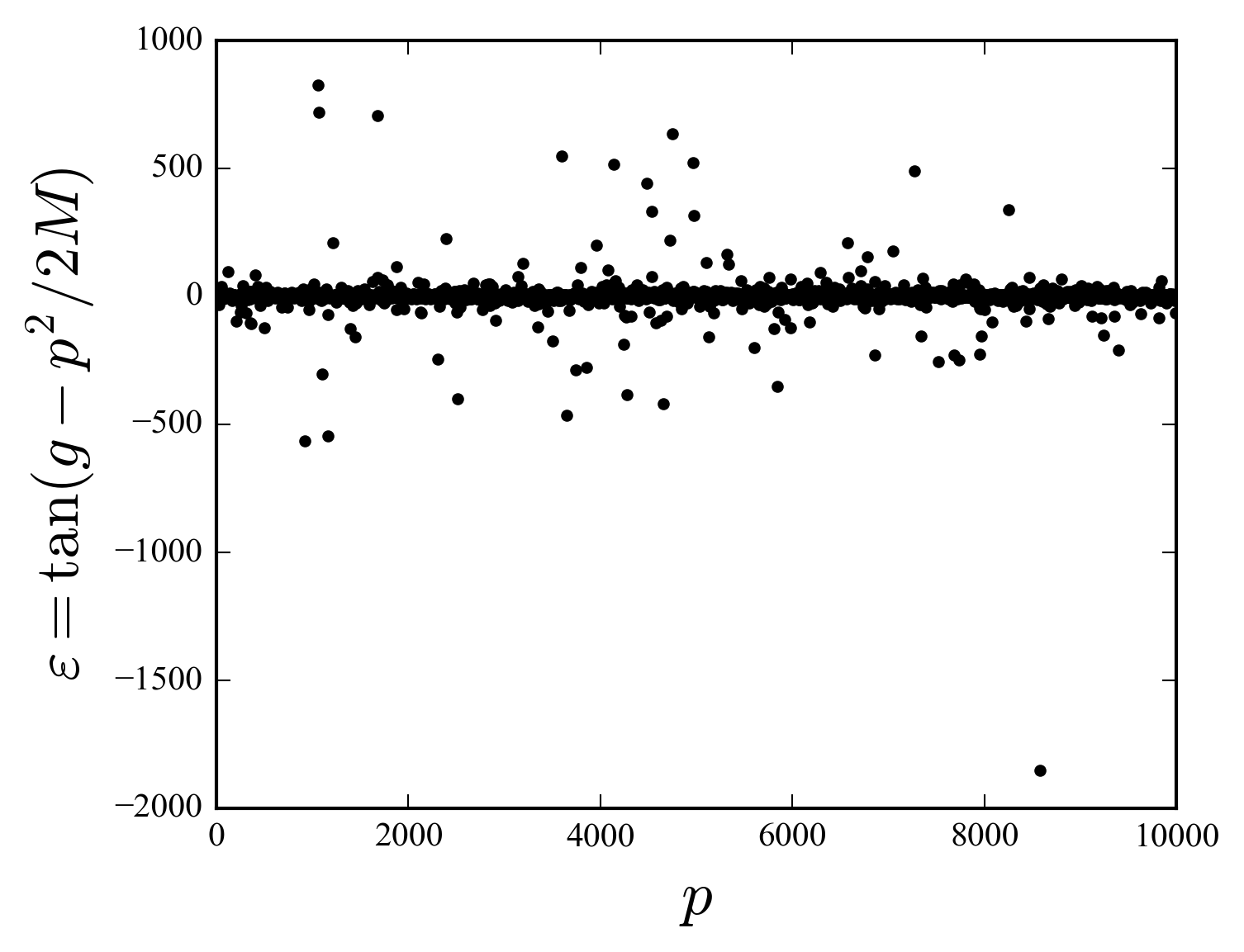
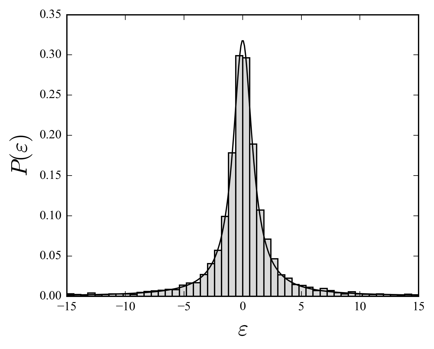
The figures (above) show the values of $\varepsilon_n$ for $\phi$ the golden ratio and $M=4$, together with its histogram, which fits a Lorentzian function.

Localization length and density of states

When restricted to nearest neighbors hopping, equation ($\ref{alDiff}$) is analogous to the Anderson model Schrödinger equation:

\begin{equation} \varphi_{n+1} + \varphi_{n-1} + (E - \varepsilon_n) \varphi_n = 0 \,, \quad P(\varepsilon_n) = \frac{W}{2\pi} \frac{1}{ \left(\frac{W}{2} \right)^2 + \varepsilon_n^2} \label{alDiffn} \end{equation}

where hopping is in momentum space instead of position space, and site disorder is distributed according to the Cauchy law, rather than uniform, law. The assumption of hopping to the neighbors is not really satisfied when $k$ is large: the integral $W_n$ is oscillating and decays slowly; however, this approximation can give us a relevant qualitative information about the localized states of the kicked rotator.

To compute the ensemble-averaged Lyapunov exponent, or equivalently the inverse of the localization length $\overline{\lambda} = 1/\ell$, we can solve ($\ref{alDiffn}$) as an initial value problem, fixing $\varphi_0$ and $\varphi_1$, to find $\varphi_L(E) \sim \E^{L/\ell(E)}$ (if $E$ is not in the spectrum, according to the Furstenberg theorem). In one dimension $\varphi_L(E)$ is a polynomial of degree $L-1$ whose zeros correspond to the eigenvalues of the chain with fixed boundary $\varphi_L=0$. This is special for one dimension, because we can order the eigenmodes by their number of nodes: the lowest energy state has no nodes, one node for the first “excited” state, etc. This is a property that the disorder do not change. Therefore, we can write,

\begin{equation} \varphi_L(E) = C \prod_{k=1}^{L-1}(E_k - E)\,, \quad \ln \varphi_L(E) = \sum_{k=1}^{L-1} \left[ \ln |E_k -E| + \I \pi \theta(E - E_k) + \ln C \right]\,, \end{equation}

where indices $k,\ldots$ denote energy levels ($n,\ldots$, are for “position”); the second expression takes into account the sign change at each node, which introduces a jump of $\I \pi$ in the logarithm ($C$ is a normalization constant). In the limit of an infinite system, the sum over states can be replaced by an integral over the density of states; separating real an imaginary parts, we obtains,

\begin{equation} \frac{1}{\ell} = \lim_{L\rightarrow \infty} \frac{1}{L} \mathrm{Re}\, \overline{ \varphi_L(E) } = \int_{-\infty}^{\infty} \Di{E'} \overline{\rho(E')} \ln | E - E'| + \ln 2\,, \label{alHJT} \end{equation}

and,

\begin{equation} F(E) = \lim_{L\rightarrow \infty} \frac{1}{\pi} \mathrm{Im}\,\overline{ \varphi_L(E)} = \int_{-\infty}^{E} \Di{E'} \overline{ \rho(E')} \,, \end{equation}

where $\overline{\rho(E)}$ is the averaged density of states, and $F(E)$ is its cumulative distribution (we denote $\overline{\cdots}$, the disorder average). The constant was determined from the condition $\ell^{-1}=0$ for the free system. Equation ($\ref{alHJT}$) relates the density of states in one dimension to the localization length, it is known as the Herbert, Jones, Thouless formula.

An equivalent formula of the localization can be obtained from the behavior of the eigenstates. From ($\ref{alDiffn}$) we can deduce the form of an effective Hamiltonian, whose matrix elements are

\begin{equation} H_{nm} = \varepsilon_n \delta_{nm} - \delta_{n,m+1} - \delta_{n,m-1}\,, \end{equation}

a tridiagonal matrix, with random elements on the diagonal. We note $u_n(E_k)$ the eigenvector of eigenvalue $E_k$ of $H$. An explicit solution of the tridiagonal system is obtained from the Green function $G = (E-H)^{-1}$, whose matrix elements can be written in terms of the cofactor $C$ and determinant of the $E-H$ matrix:

\begin{equation} G=\frac{C^T(E-H)}{\det(E-H)}\,, \quad G_{nm} = \frac{ (-1)^{n+m} \det(E-H)_{mn} }{\det(E-H)} \end{equation}

where $\det_{mn}$ is the minor of row $m$ and column $n$. The computation of the minor involving the initial site $n=1$ and the last one $n=L$ is trivial for a tridiagonal matrix:

\begin{equation} G_{1L} = \prod_{k=1}^{L} (E-E_k)^{-1} \label{e:alG1L} \end{equation}

From the general form of the Green function in terms of the Hamiltonian basis functions $u_n(E_k)$,

\begin{equation} G_{1L} = \sum_k \frac{u_1(E_k) u_L(E_k) }{E - E_k}\,, \end{equation}

we find that the residue of the pole at $E=E_k$ is $u_1(E_k) u_L(E_k)$, and comparing with the residue of ($\ref{alG1L}$), we get

\begin{equation} u_1(E_k) u_L(E_k) = \prod_{j\ne k}^{L} (E_k-E_j)^{-1}\,. \end{equation}

For a Bloch-type state $|u_1u_L|\sim 1/L$, while for a localized state $|u_1u_L|\sim \E^{-L/\ell}$. Therefore,

$$\frac{1}{L} |\ln|u_1 u_L| \sim - \frac{1}{\ell}\,,$$

is finite for a localized state, but vanishes for an extended state. Therefore, taking the logarithm and passing to the continuous limit, one obtains an equivalent to formula ($\ref{alHJT}$).

Localization length of the kicked rotator

To evaluate the localization length for the Cauchy distribution,the appropriated probability law for the kicked rotator, we must calculate the average over disorder of the density of states. Instead of working directly with $\rho$, it is easier to study the Green function before, and deduce the system’s properties from the Green function. For instance, starting from the formula of the trace,

$$\mathrm{Tr}\,G(E \pm \I o) = \sum_k \frac{1}{E - E_k \pm \I o} \rightarrow P \int \Di{E'} \frac{\rho(E')}{E-E'} \mp \I \pi \rho(E)$$

$P$ stands for the principal value and $o\rightarrow 0$, it is easy to demonstrate that the derivative of the Lyapunov exponent is given by

\begin{equation} \frac{\partial }{\partial E} \overline{ \lambda(E)} = \mathrm{Re}\, \mathrm{Tr}\, \overline{ G(E + \I o )} \,, \quad \overline{ \rho(E)} = \frac{-1}{\pi} \mathrm{Im}\, \overline{G(E + \I o )} \,. \label{alGa} \end{equation}

Therefore, we need to average the Green function. One of the most interesting (and generally applicable) methods to compute disorder averages in many-body systems is the replica method devised by Edwards and Anderson (1975) [see the book Peliti, “Statistical Mechanics in a Nutshell” (2011)].

The idea of the replica method comes from the statistical mechanics of disordered systems as a trick to compute the disorder averaging $\overline{\cdots}$ of the free energy:

$$ \overline{F} = \lim_{N\rightarrow\infty} - T\overline{\ln Z} = \lim_{R \rightarrow 0} \lim_{N \rightarrow \infty} -T \frac{ \overline{Z^R} -1 }{R} $$

(note the intervention of the limits). Instead of computing the average of a logarithm, which is almost never possible, one computes the moments $\overline{Z^R}$ for integer $R$, and then analytically continue to $R \rightarrow 0$, in the thermodynamic limit.

In order to calculate the averaged Green function ($\ref{alGa}$), we write it as a Gaussian integral,

\begin{equation} G_{nm} = \langle n|G(E+\I o)|m\rangle = \frac{2}{Z} \int_{-\infty}^{\infty} \mathrm{D}\varphi \,\varphi_n \varphi_m \exp \left[-\I \varphi^T ( E-H+\I o ) \varphi \right] \,, \end{equation}

where $\mathrm{D} \varphi = \prod_{i=1}^{L}\Di{\varphi_i}$, and $\varphi = (\varphi_1,\ldots,\varphi_L)$ is the (real) vector of integration variables; the normalization factor is,

$$Z = \frac{\pi^{L/2}}{ \det(E - H + \I o)^{1/2} }\,. $$

If we replicate now the integral $R$ times and average over disorder, the normalization factor $Z^R$ will disappear in the limit $R\rightarrow 0$:

\begin{equation} \overline{G_{nm}} = 2 \lim_{R\rightarrow0} \int \mathrm{D}\varepsilon P[\varepsilon] \prod_{r=1}^{R} \int_{-\infty}^{\infty} \mathrm{D}\varphi^r \,\varphi_n^r \varphi_m^r \exp \left[-\I \varphi^{rT} \left( E-H[\varepsilon]+\I o \right) \varphi^r \right] \,, \label{alGrm} \end{equation}

where we explicitly noted the dependency of the Hamiltonian on the random vector $\varepsilon$ of site disorder energies. The remarkable point about the Cauchy distributed disorder, is that the integral over the Lorentzian gives an exponential function, which naturally adds to form an effective disorder averaged Hamiltonian. Indeed, because of the independence of random energies, the term in $\varepsilon_n$ of $H$ can be integrated separately,

$$ \frac{W}{2\pi} \int_{-\infty}^{\infty} \Di{\varepsilon_n} \frac{\E^{\I \varphi_n\, \varepsilon_n\, \varphi_n}}{(W/2)^2 + \varepsilon_n^2}= \E^{-W \varphi_n^2/2} $$

which results formally in replacing $\varepsilon_n \rightarrow \I W/2$ in $H$, to obtain from the final expression of $G$, the effective Hamiltonian:

\begin{equation} \overline{G(E+ \I o)} = \frac{1}{E- \overline{H} +\I o}\,, \quad \overline{H_{nm}} = \frac{\I W}{2} \delta_{n,m} - \delta_{n,m+1} - \delta_{n,m-1} \end{equation}

The noteworthy point is that this effective Hamiltonian is a non-hermitian operator, underlining the “dissipative” aspect of the disorder.

We need now to compute,

\begin{equation} \mathrm{Tr}\, G = \sum_m \frac{\det(E-\overline{H})_{mm}}{\det(E-\overline{H})}\,. \end{equation}

the resulting expression of the integral ($\ref{alGrm}$). This equation is conveniently written using the well known matrix formula $\mathrm{Tr}\,\ln M = \ln \det M$, for any matrix $M$:

$$\mathrm{Tr}\, G = \frac{\partial}{\partial E} \ln \det(E - \overline{H})\,,$$

which reduces the problem to the standard problem of computing the determinant of a tridiagonal matrix $D_L = \det(E - \overline{H})$. It is obtained by simple recursion:

\begin{align*} D_0 &= 1 \\ D_1 &= E - \frac{\I W}{2} \\ D_2 &= (E - \frac{\I W}{2})^2 - 1 \\ D_n &= (E - \frac{\I W}{2} )D_{n-1} - D_{n-2}\,. \end{align*}

The ansatz $D_n\sim x^n$, gives the two solutions

$$x_\pm = \frac{1}{2} \left[ E-\frac{\I W}{2} \pm \sqrt{(E-\I W/2)^2 - 4} \right]\,$$

which leads to

$$D_L = \frac{x_+^{L+1} - x_-^{L+1} }{x_+ - x_-}\,.$$

In the $L\rightarrow\infty$ limit, only the larger root survives. The final expression for the localization length is,

\begin{equation} \frac{1}{\ell(E)} = \ln \frac{1}{2}\left| E-\I W/2 + \sqrt{(E-\I W/2)^2 - 4} \right|\,, \end{equation}

or, in a more explicit form:

\begin{equation} \cosh\left[ \frac{2}{\ell(E)} \right] = \frac{1}{4} \left( E^2 + \frac{W^2}{4} \right)+ \frac{1}{4} \left[(E+2)^2 + \frac{W^2}{4} \right]^{1/2} \left[(E-2)^2 + \frac{W^2}{4} \right]^{1/2} \,. \end{equation}

We observe that when the hopping energy dominates (in the present units this corresponds to $E\rightarrow0$ and $W\rightarrow0$), the localization length diverges, and that for any value of $W>0$, $\ell(E)$ is finite, in accordance with the phenomenology of the kicked rotator.

»quantum chaos »kicked rotator »random matrices »quantum walk