$\newcommand{\I}{\mathrm{i}} \newcommand{\E}{\mathrm{e}} \newcommand{\D}{\mathop{}\!\mathrm{d}} \newcommand{\Di}[1]{\mathop{}\!\mathrm{d}#1\,} \newcommand{\Dd}[1]{\frac{\mathop{}\!\mathrm{d}}{\mathop{}\!\mathrm{d}#1}}$

»quantum chaos »dynamical localization »random matrices »quantum walk

Kicked rotator

The evolution of a time dependent quantum system $H(t)$, initially in state $|\psi(0) \rangle$,

$$ \I \frac{\partial }{\partial t} |\psi(t)\rangle = H(t) |\psi(t)\rangle $$

($\hbar=1$) can be described by an unitary operator $U(t)$,

$$|\psi(t) \rangle = U(t) |\psi(0)\rangle\,,\quad U(t) = \mathrm{T} \exp\left(-\I \int_0^t \Di{s} H(s) \right)\,, $$

where $\mathrm{T}$ is the time ordering operator. In the important case of periodic systems $H(t+T) = H(t)$, of period $T$, the Floquet operator $F$ gives a stroboscopic view of the quantum dynamics:

$$F=U(T)\,, \quad |\psi(nT)\rangle = F^n |\psi(0)\rangle\,. $$

The eigenvectors of $F$ form a suitable basis to represent the quantum state $|\psi(nT)\rangle$:

$$F |\phi_k \rangle = \E^{-\I \phi_k} | \phi_k \rangle\,,\quad \psi(nT) = \sum_k \E^{-\I n \phi_k} \langle\phi_k |\psi(0)\rangle |\phi_k\rangle\,, $$

where $\phi_k$ are the eigenphases (or “quasi-energies”). In the particular case where the system is perturbed by a train of instantaneous kicks, the Hamiltonian is of the form:

$$H(t) = H_0 + V \sum_{-\infty}^{\infty} \delta(t - nT)\,, $$

where $H_0$ is the unperturbed system, the Floquet operator splits into two exponential factors:

$$F = \E^{-\I V} \E^{-\I H_0 T}\,,$$

here $V$ is the perturbation, it has the dimensions of an action, and may depend on the position, spin or other observables. $F$ describes the motion of the quantum system just after a kick, up to after the following kick.

Exercise

Show that the splitting of the Floquet operator is valid in the limit $\Delta t \rightarrow 0$ for a general pulsed system
$$H(t) = H \begin{cases} H_0, &\text{ if } nT < t < (n+1)T-\Delta t\\ H_0 + V/\Delta t, &\text{ if } (n+1)T-\Delta t < t < (n+1)T \end{cases}\,.$$

The Hamiltonian of a kicked rotator is defined as the quantum version of the standard map classical Hamiltonian:

\begin{equation} H = \frac{L_z^2}{2I} - JT \cos \varphi \, \delta_T(t) \end{equation}

where the operators $L_z$ and $\varphi$ correspond to the $z$ component of the angular momentum and the angular direction in the perpendicular plane of the rotator, respectively; $I$ is the inertia moment, $T$ the kicking period, $J$ is an energy constant, and $\delta_T$ is the periodic Dirac function of period $T$. The first term represent the unperturbed rotation, and the second one the time $t$ dependent perturbation. This model is suitable to describe the physics of ionization Rydberg states of the hydrogen atom in a microwave field, or laser excited ultracold trapped atoms, or nitrogen atoms kicked by a train of laser femtosecond pulses [Floss (2015) PRL 115, 203002]

From the set of parameters it is possible to form two nondimensional quantities:

$$ M = \frac{I}{\hbar T}\,, \quad k = \frac{J T}{\hbar} $$

Without loss of generality we can take $\hbar=T=1$. Using these units the nondimensional Hamiltonian (in units of energy $\hbar/T$), writes

\begin{equation} \label{krH} H = \frac{p^2}{2M} + k \cos x \, \delta_1(t)\,, \end{equation}

where we denoted $p = L_z/\hbar$ and $x=\varphi \in (0,2\pi)$, which satisfy the usual commutation rule $[x,p]=\I$. The Heisenberg equations derived from this Hamiltonian are equivalent to the classical standard map with momentum $P= p/M$ and coupling constant $K=k/M$; the classical limit is obtained for very large $(k,M) \rightarrow \infty$, keeping $K=\text{const}$. Hoewever, major difference remains, in the quantum case the problem has a second nondimensional parameter, not present in the classical case, that manifests itself in the commutation relation $[P,x] = \I/M$. Therefore, the parameter $M$ is the inverse of an effective Planck constant: it controls the amplitude of quantum fluctuations.

The evolution operator for one time period $T=1$, the so-called Floquet unitary operator $F$, is given by

\begin{equation} \label{krF} F = \E^{-\I k \cos x} \, \E^{-\I p^2/2M}\,, \quad | \psi(t+1) \rangle = F | \psi(t) \rangle \end{equation}

In momentum representation, the eigenvalues of the operator $p$ are integer numbers $n \in \mathbb{Z}$, and the base functions are the kets $|n\rangle$ satisfying

\begin{equation} \label{krpx} p |n\rangle = n |n\rangle\,, \quad \langle x| n\rangle = \frac{\E^{\I n x}}{\sqrt{2\pi}}\,, \end{equation}

where $|x\rangle$ is a complete basis of the $x$ operator

$$ \int_{0}^{2\pi} \Di{x} |x\rangle \langle x| = 1\,. $$

Using these definitions it is straightforward to find an explicit expression for the Floquet operator in the angular momentum base:

\begin{equation} \label{krFn} \langle n | F | m \rangle = \E^{-\I m^2/2M}\, \I^{m-n}\, J_{m-n}(k)\,, \end{equation}

where $J_n(k)$ is the Bessel function of order $n$:

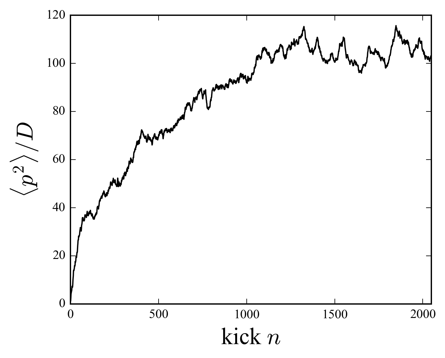
$$ J_n(z) = \frac{1}{\I^n \pi} \int_{0}^{\pi} \Di{\theta} \cos(n \theta) \, \E^{\I z \cos \theta}\,. $$

Within the momentum representation we can compute the expected value of $p^2$, in order to compare it with the behavior of the classical system; for $k$ large enough we expect a diffusion regime characterized by a diffusion coefficient $D=k^2/2$. After $L$ kicks the initial state $|\psi_0\rangle$ hop to $\psi(t)$:

\begin{align} \langle \psi(t)|p^2|\psi(t)\rangle & = \langle \psi_0 | F^{\dagger t} p^2 F^t | \psi_0 \rangle \nonumber\\ & = \sum_{p,n,m} \langle \psi_0| n \rangle \langle n | F^{\dagger t} | p \rangle p^2 \langle p | F^{\dagger t} | m \rangle \langle m | \psi_0 \rangle \nonumber\\ & = \sum_{p,n,m} p^2 \psi^*_{0n} F^{\dagger t}_{np} F^t_{pm} \psi_{0m} \end{align}

where $F$ is given by ($\ref{krFn}$). This analytic (exact) expression for the second moment of the angular momentum probability distribution, is in fact useless. It is a sum over $\mathbb{Z}^3$ of highly oscillating functions, any truncation may give rise to uncontrolled errors. To compute $\langle p^2\rangle$ we need a smarter numerical method.

Numerical code

iterates bifurcations

To compute the evolution of the rotator, we use equation ($\ref{krF}$), which is much more efficient than the evaluation of the Bessel’s sums [Izrailev (1990), Phys. Rep. 196, 299]. The Floquet operator is splitted into the kinetic term in angular momentum representation, and the potential part, in position representation. The change of representation is computed by fast fourier transforms (the transformation functions between the two representations ($\ref{krpx}$) are plane waves). The figures show the results of a simulation with $k=20$ and $M=4$.

def krt(T, K, M, DIAG = 10):
    """Quantum kicked rotartor: computes w = <p^2> and psi

    Initial state $p[0] = 1$
    Output:
        w   : the variance of the angular momentum as
              a function of time
        p   : array with the momentum eigenvalues, 
              in the interval (-T,T), integers
        psi : the wavefunction in momentum representation
              array of shape (N=2T, T/DIAG)
    """
    N = 2*T
    p = fftfreq(N, 1.0/N)
    x = arange(0, 2*pi, 2*pi/N)
    #
    Up = exp(-1j*p**2/(2*M))
    Ux = exp(-1j*K*cos(x))
    #
    psi = zeros((N, T//DIAG + 1), dtype = complex)
    psi_t = zeros(N, dtype = complex)
    psi_t[0] = 1
    #
    w = zeros(T)
    it = 1
    for t in range(T):
        psi_t = fft(Ux * ifft(Up * psi_t))
        w[t] = sum(p**2 * abs(psi_t)**2)
        if t%DIAG == 0:
            psi[:,it] = psi_t
            it += 1
    return w, fftshift(p), fftshift(psi)

Exercice

Compute the (classical) quasilinear diffusion coefficient for the standard map:
$$ p_{n+1} = p_n + k \sin x_n\,, \quad x_{n+1} = x_n + p_{n+1}/M $$

Solution:

In the quasilinear approximation (valid in the global chaotic regime) we assume the angle $x \sim \mathcal{U}(0,2\pi)$, uniformly distributed on the circle:

\begin{align*} \langle (p_t - p_0)^2 \rangle &= \big\langle \big[ \sum_n (p_{n+1} - p_n) \big]^2 \big\rangle \\ & = \sum_{m,n} \langle (p_{m+1} - p_m) (p_{n+1} - p_n) \rangle \\ & = k^2 \sum_{m,n} \langle \sin x_m \sin x_n \rangle \end{align*}

Using the integral:

$$ \int_{0}^{2\pi} \frac{\Di{x_m}}{2\pi}\frac{\Di{x_n}}{2\pi} \sin x_m \sin x_n = \frac{1}{2} \delta_{m,n} $$

we obtain the quasilinear diffusion coefficient:

$$ D = \frac{k^2}{2}$$

Results

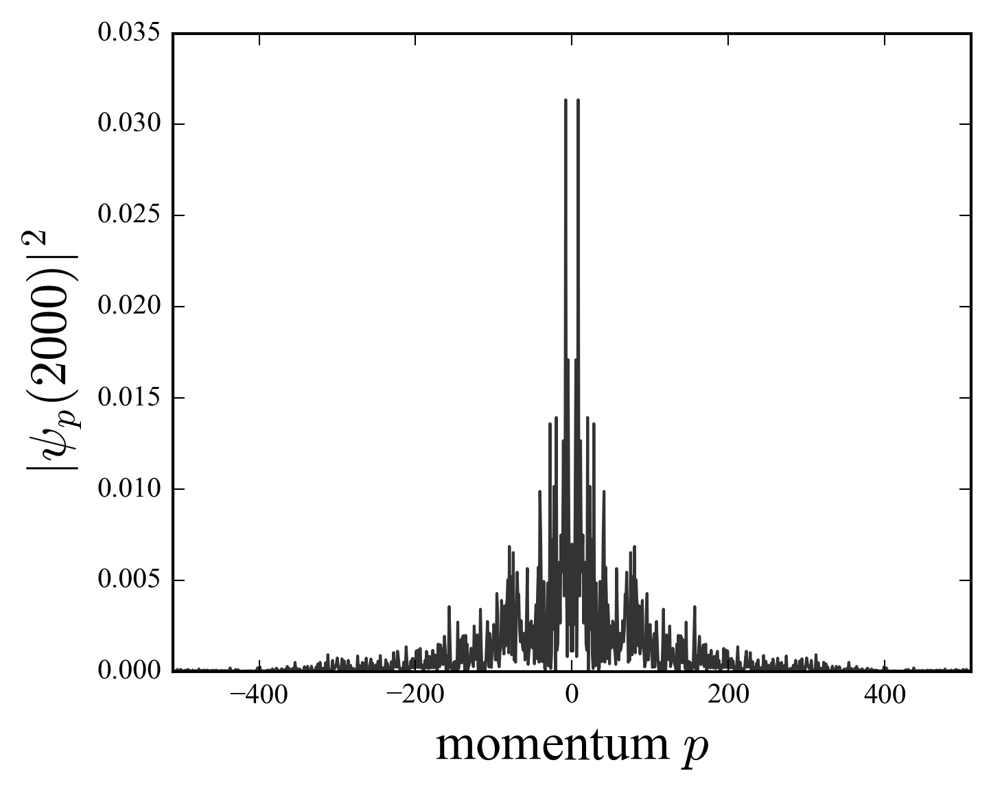
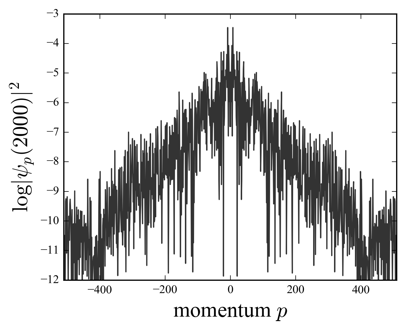
The numerical results (figure) show that the behavior of the quantum systems is strikingly different, even for large $K=k/M$, to its classical counterpart. The simulation parameters are $k=20$, $M=4$, $K=k/M=5$. After an initial transient where both systems follow the diffusion law, a significant departure arises: the quantum evolution tends to saturation $\langle p^2 \rangle \rightarrow \text{const.}$ and quantum diffusion is stopped. This phenomenon, discovered by Casati et al (1979) and known as quantum suppression of classical chaos, can be attributed to the localization of the wave function, as seen in the figure, where the logarithmic scale reveals exponential tails.

Bibiliography

Lévi et al. (2003) Quantum computing of quantum chaos in the kicked rotator model, Phys. Rev. E 64, 046220 (2003)

»quantum chaos »dynamical localization »random matrices »quantum walk