Map | Random physics

$\newcommand{\I}{\mathrm{i}} \newcommand{\E}{\mathrm{e}} \newcommand{\D}{\mathop{}\!\mathrm{d}} \newcommand{\Di}[1]{\mathop{}\!\mathrm{d}#1\,} \newcommand{\Dd}[1]{\frac{\mathop{}\!\mathrm{d}}{\mathop{}\!\mathrm{d}#1}}$

»chaos »stability »hamiltonian systems »plasmas

Chaos

The intuitive notions of regular and irregular, smooth and rough, predictable and unpredictable, can be illustrated by the behavior of an analytic function (regular) compared with the Weierstrass function $W$ of the real variable $x$ (irregular),

\begin{equation} \label{wx} W(x) = \sum_{n=0}^\infty \frac{\cos(3^n\pi x)}{2^n}\,,\quad x \in [-2,2]\,, \end{equation}

which is continuous but nowhere differentiable. The non differentiability of $W$ can be grasped form the divergence of the series:

$$ \sum_{n=0}^\infty \frac{3^n}{2^n}\,. $$

and the fact that $\cos(x)$ is bounded. As a consequence, the graph of $W$ do not possess a tangent at any point. The graph is then nowhere smooth.

The Weierstrass function is continuous, periodic and even; it is nowhere derivable, and possesses a fractal structure: the insets are zooms over the successive circled regions.

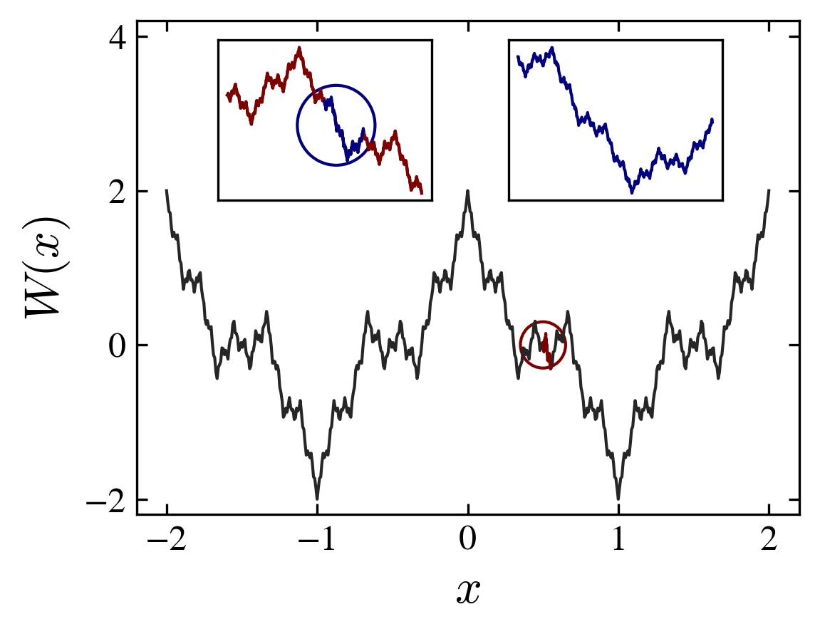
The irregularity of function’s graph can be qualitatively associated to the existence of a large range of scales. Indeed, if we zoom the curve around any point, we discover that the zoomed graph has as many features as the original one. This self-similar structure was called fractal by Mandelbrot. The fractal dimension $D$ of ($\ref{wx}$) is,

$$ D = 2 - \frac{\ln 2}{\ln 3}\,, $$

in between $D=1$ the dimension of a (smooth) line, and $D=2$ the dimension of a surface.

Other intuitive idea is that irregular and unpredictable are forms of randomness, like the sequence of heads and tails obtained by tossing a coin. However, simple deterministic systems show erratic behavior. One example is the Bernoulli shift:

\begin{equation} \label{x2x} x_{n+1} = B(x_n) = 2x_n \mod{1}, \quad x \in [0,1]\,,\; n=0,1,\ldots \end{equation}

which gives a sequence of real numbers whose leading bit, in their binary representation, is dropped at each step $n$:

$$ x_n = 0.11000101001110\ldots \;\rightarrow\; x_{n+1} = 0.1000101001110\ldots\,. $$

The sequence thus obtained can be trivial if the seed $x_0 \in \mathbb{Q}$ is rational, but for a generic irrational number it is random: it is impossible to correctly gess the next number in the series from the knowledge of the actual one (or even the whole history), the sequence is unpredictable. We can prove that the density distribution $\rho(x)$ of the values of $x$ is uniform on the interval $[0,1]$, using the Perron-Frobenius operator:

\begin{equation} \label{pf} \rho(x) = \int_0^1 \D y \, \delta(x - B(y))\rho(y)\,. \end{equation}

Indeed, separating the interval in $x<1/2$ and $x>1/2$, we get

$$ \int_0^{1/2} \D y \, \delta(x - 2y))\rho(y) = \frac{1}{2}\rho \left(\frac{x}{2}\right)\,, $$

where we applied the formula

$$ \delta(f(x)) = \sum_{x_0 \in \{f(x_0)=0\}} \frac{\delta(x-x_0)}{|f'(x_0)|}\,, $$

and,

$$ \int_{1/2}^{1} \D y \, \delta(x - 2y + 1))\rho(y) = \frac{1}{2}\rho \left(\frac{x+1}{2}\right)\,, $$

from which we obtain an equation for the function $\rho$:

$$ \rho(x) = \frac{1}{2} \rho\left(\frac{x}{2}\right) + \frac{1}{2}\rho \left(\frac{x+1}{2}\right)\,. $$

The solution of this equations is precisely the uniform distribution $\rho(x) = 1$. This establishes the equivalence of the “dynamical system” ($\ref{x2x}$) with the coin tossing game. In some sense, randomness is at the heart of numbers!

This randomness in numbers is also surprisingly displayed by the zeros of the Riemann zeta function $\zeta(s)$ on the imaginary line at $s=1/2$. The zeta function is defined by the series,

\begin{equation} \label{zeta} \zeta(s)=\sum_{n=1}^\infty \frac{1}{n^s} = \prod_p \frac{1}{1-p^{-s}} \,, \quad s>1 \end{equation}

where the second formula, the product over prime numbers $p$, due to Euler, derives from the fact that every integer can be factored in a product of primes (fundamental theorem of arithmetic). Its analytic continuation $s\in\mathbb{C}$, obtained by Riemann in his famous paper where he found an exact expression for the distribution of prime numbers (Riemann, 1859), is given by,

\begin{equation} \label{zetaC} \zeta(s) = \frac{\Gamma(1-s)}{2\pi \I} \int_{\infty + \I0}^{\infty - \I0}\frac{\D z}{z} \frac{(-z)^{s}}{\E^z-1} \end{equation}

where the contour encloses the origin in the counterclockwise direction. The integral converges for arbitrary complex $s\ne 1$, where $\zeta$ has a simple pole. Riemann also proved the functional relation

\begin{equation} \label{zetaac} \zeta(s) = 2^s \pi^{s-1} \sin (\pi s/2)\, \Gamma(1-s)\zeta(1-s)\,, \end{equation}

which allows to find the values of $\zeta(s)$ for $s \ne 0, 1$. The change of sign of the real function,

\begin{equation} \label{Z} Z(t) = \E^{\I \vartheta(t)} \zeta\big(\tfrac{1}{2} + \I t\big)\,,\quad \vartheta(t) = \mathrm{Im}\, \ln\Gamma\left(\tfrac{1}{4}+\tfrac{1}{2}\I t\right) - \tfrac{1}{2}\ln (\pi)\,t \end{equation}

gives the zeros of $\zeta$ on the critical line ($s=1/2+\I t$, with $t\in\mathbb{R}$). Riemann computed the mean number of zeros in the interval $(0,t)$:

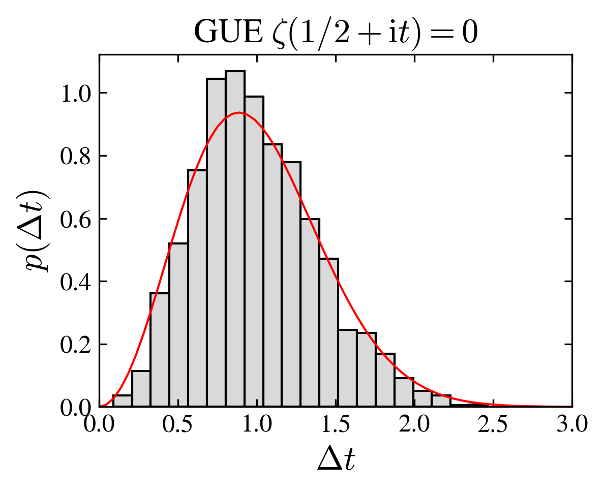
$$ N(t) \approx \frac{\vartheta(t)}{\pi} \approx \frac{t}{2\pi}\ln \frac{t}{2\pi} - \frac{t}{2\pi} - \frac{1}{8} $$

It is a remarkable fact that the gaps between consecutive zeroes are distributed according to the law governing the energy level spacing of a random hermitian matrix. Indeed, after an appropriate normalization to eliminate the mean trend, the separation between zeros,

$$ \Delta_n = \frac{t_{n+1} - t_n}{2\pi}\ln \frac{t_n}{2\pi} $$

follows the distribution of a gaussian unitary ensemble matrix (GUE), as can be seen in the figure below.

Histogram of the gaps $\Delta_n$ between consecutive zeros on the critical line, for $n=1,\ldots,5596$. Detailed calculations using up to $10^{13}$ zeros, give a perfect fit to the gaussian unitary ensemble (GUE) (Gourdon, 2004).

Dynamical systems

The state of a physical system $O$ is determined by a set of variables $X$ and parameters $M$, together noted $o=\{X,M\}$; $o$ represents one state of the system $O$. Physical laws do not depend on units, therefore the set $M$ is nondimensional.

In a dynamical system we distinguish the time parameter $t$ on which the state depends $o = o(t) \in O$. If $t \in T = \mathbb{R}$ the system’s evolution is continuous; if $t \in T = \mathbb{Z}$ it is discrete. The time trajectory $o(t)$ is generated by the one-parameter flow operator $F_t$:

\begin{equation} o(t) = F_t \, o(0) \,, \quad F_{t_1} \circ F_{t_2} = F_{t_1 + t_2} \end{equation}

where $o(0)$ is the initial state (the state at $t=0$). At variance with variables $X$ that depend on time, the set $M$ of parameters on which $F$ depends, are considered fixed (independent of $t$)

$$ o(t) \equiv X_M(t)\,. $$

The history $X= X_M(t)$ is called the “trajectory” or orbit of the dynamical system and the space spaned by $X$ the “phase space”. If $F$ is invertible, then the flow has a group structure.

Examples:

Newton dynamics is governed by the law relating force with acceleration,
\begin{equation} m\frac{\D^2 \boldsymbol{x}}{\D t^2} = - \Dd{\boldsymbol{x}} V(\boldsymbol{x}) \,, \end{equation}
which gives the trajectory $\boldsymbol{x} = \boldsymbol{x}(t)$ for a particle of mass $m$ in a potential $V$. This ordinary differential equation trivially generalizes to a system of particles. In terms of the phase space vector $z=(x,p)$ and the Hamiltonian $H=H(z)$ the above equation can be written as:
\begin{equation} \dot{z} = \Omega \frac{\partial }{\partial z} H \end{equation}
where $\Omega$ is the symplectic matrix
$$ \begin{pmatrix} 0 & 1 \\ -1 & 0 \end{pmatrix}\,, $$
here $1$ is the identity matrix, based on the dimension of the configuration space $\mathrm{dim}\,x$, and $\partial/\partial z$ is the gradient vector.
Quantum mechanics. A quantum system defined by a Hamiltonian $H$ evolves in time according to the Schrödinger equation,
\begin{equation} |\psi(t) \rangle = U(t,0) | \psi(0) \rangle \,, \end{equation}
where $| \psi \rangle$ is the quantum state (a vector in Hilbert space) and the operator $U$ is given by ($\hbar = 1$),
$$ U = \E^{-\I H t}, $$
in the case of $H$ independent of time. As a consquence of the hermicity of $H=H^\dagger$, the evolution is unitary $U^{-1}=U^\dagger$ (even if $H=H(t)$). Quantum dynamics is invertible.

The logistic map

A simple and rich dynamical system is the logistic map,

\begin{equation} x_{n+1} = \mu x_n (1 - x_n)\,, \quad n = 0,1,2,\ldots \end{equation}

Depending on the value of the parameter $\mu \in [0,4]$, the iterates $x_n$ can tend towards a fixed point $x^* = x_{n+1} = F_1(x_n) = x_n$, a periodic orbit $x_{n+p} = F_p(x_n) = x_n$, of period $p$, or for most values $\mu > \mu_\infty = 3.57$, chaotic. The stability of a periodic orbit is determined by the value of the derivative of the map at the fixed point (Jacobian $\D x_{n+1}/ \D x_n$); for $D[F_p](x^*)<1$ the orbit is stable.

iterates bifurcations histogram

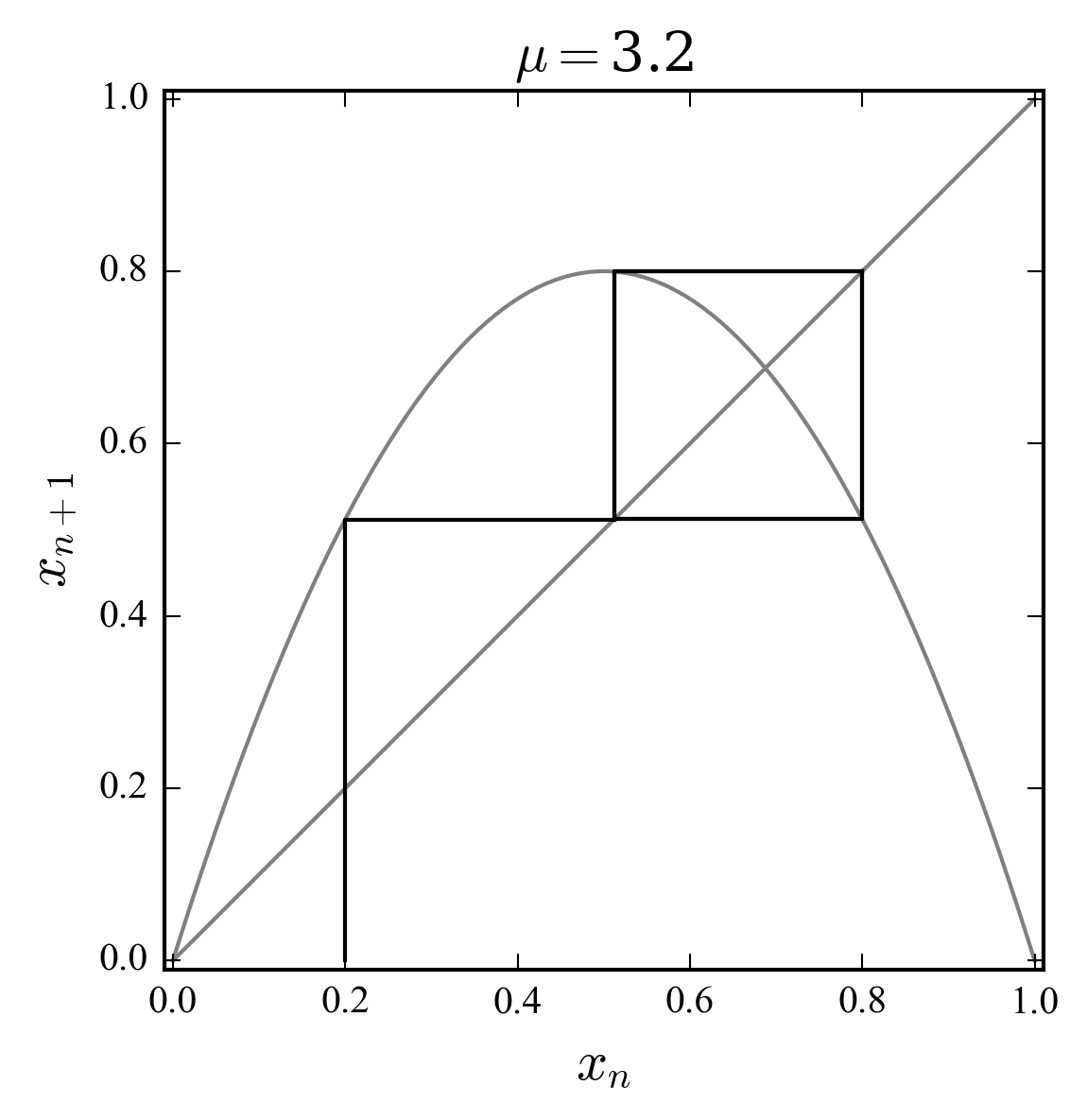
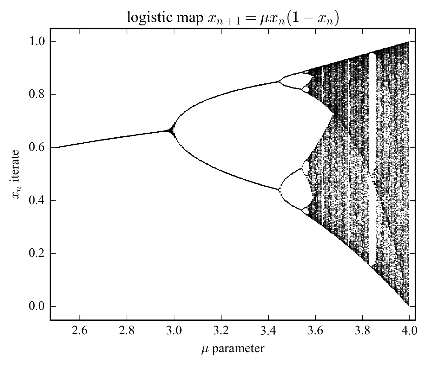
For instance, the $p=1$ fixed point becomes unstable at $\mu = 3$, from which a double periodic orbit $p=2$ sets in. Transition toward chaos is through period-doubling bifurcations, whose accumulation point ($p=2^n$ with $n \rightarrow \infty$) is just $\mu_\infty$.

Exercise: dyadic map

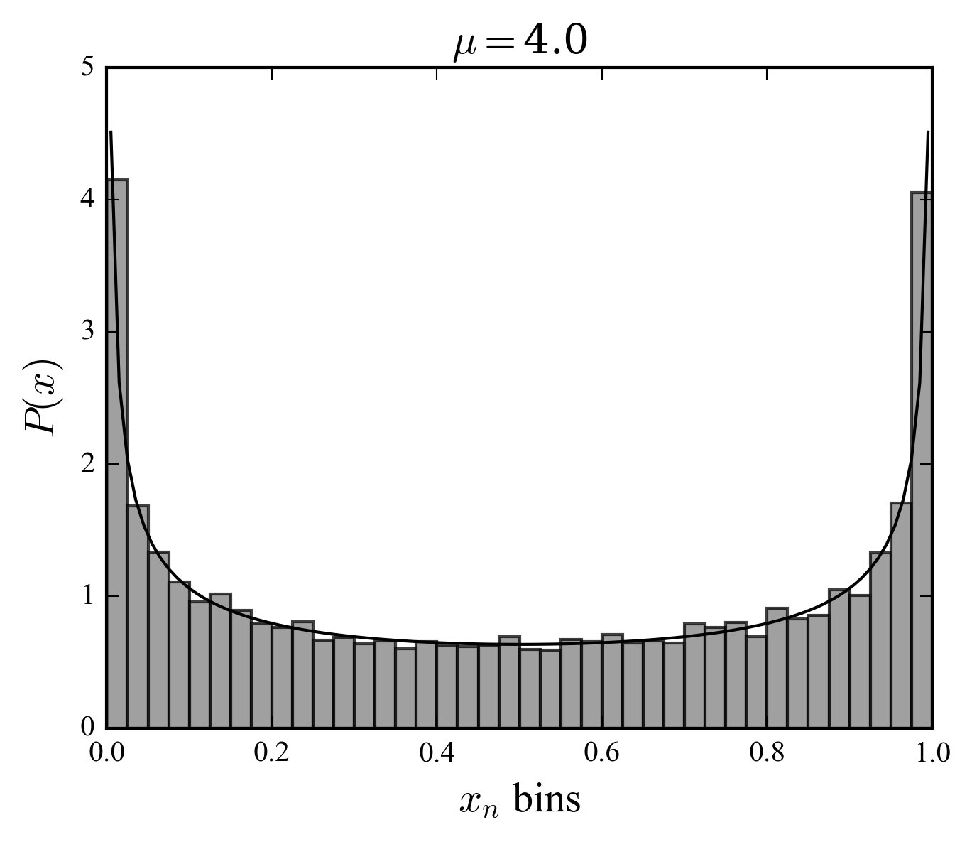
Show that the dyadic map, $x_{n+1} = 2 x_n \mod{1}$ (Bernoulli shift), is equivalent to the logistic map for $\mu=4$ and demonstrate that, in this case, the orbit is given by
$$ x_{n+1} = \sin^2 \left( \pi a 2^n \right) \,, \quad x_0 = \sin^2 \pi a $$
if the initial condition is $x_0$. * We note that for $\mu=4$ the logistic map $F$ is equivalent to the Bernoulli shift; the Bernoulli shift can be lifted to the complex unit circle: $B(z) = z^2$ with $|z|=1$. * Direct computation of $F_n(x_0)$ gives the result.

Exercise:

Investigate numerically the logistic map; show empirically the divergence of two initially close trajectories; build the bifurcation diagram; study the histogram of the iterates for $\mu = 4$ and compare with a random process.

A simple code:

"""
Logistic map:
    logistic_points(mu, n):
    x_n values of the logistic map mu*x*(1-x)
"""
def f_logistic(mu, x):
    return mu*x*(1-x)

def logistic_points(mu, n = 100):
    x = 0.2
    #
    # filter transient
    for i in range(100):
        x = f_logistic(mu, x)
    #
    # iterates
    xn = zeros(n)
    for i in range(n):
        x = f_logistic(mu, x)
        xn[i] = x
    return xn

The standard map

The discrete time map defined by,

\begin{equation} \label{sm} x_{n+1} = x_n + p_{n+1}\,, \quad p_{n+1} = p_n + K \sin x_n \end{equation}

where $(x,p)$ are position (angle) and momentum (action) modulo $2\pi$ variables, is a Hamiltonian dynamical system,

\begin{equation} \label{smh} H = \frac{p^2}{2} - K \sum_{n=-\infty}^{\infty} \cos(x - 2\pi nt) \end{equation}

as can be easily verified using the Poisson summation formula:

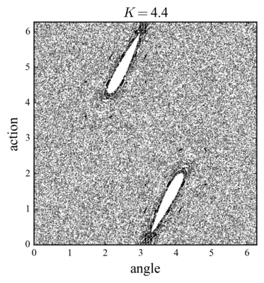
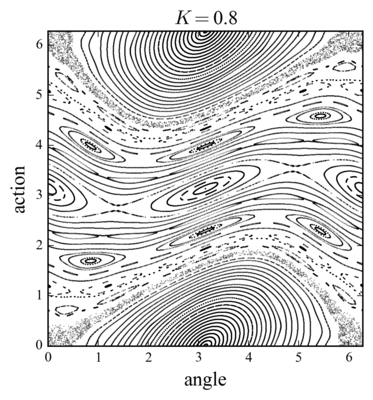
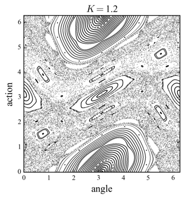
$$\sum_{n=-\infty}^{\infty} \delta(t-n) = \sum_{n=-\infty}^{\infty} \E^{\I 2\pi nt}\,.$$

Equation ($\ref{smh}$) define the Chirikov standard map, also important in quantum mechanics, which describes the transition to chaos in Hamiltonian systems. The origin of chaos is in the overlap of resonances: when the distance between the separatrices $\Delta p = 2 \sqrt{K}$ (the separatrix corresponds to $E=K$ line) becomes of the order of the resonance separation $\Delta \omega = 2\pi$. This criterion gives $K_c = \pi^2/4$; numerical evaluation gives a stochastic threshold at $K_c \approx 0.98$.

Poincaré section and monodromy matrix

The standard map is the Poincaré section of Hamiltonian ($\ref{smh}$): a section of the phase space transversal to the trajectories, such that a periodic orbit appears as a point (a double periodic orbit appears as two points, etc.).

Consider a general twodimensional $z=(x,p)$ Poincaré map $z \rightarrow z'=P(z)$; if $z$ is a fixed point

$$P(z) = z$$

then

$$ \delta z' = P(z+\delta z) - P(z) \,, \quad P(z+\delta z) = z + \D P(z) \delta z\,.$$

where the matrix $M = \D P (z)$

\begin{equation} M = \begin{pmatrix} \frac{\partial x'}{\partial x} & \frac{\partial x'}{\partial p}\\ \frac{\partial p'}{\partial x} & \frac{\partial p'}{\partial p} \end{pmatrix} \end{equation}

corresponding to the tangent map, is called the monodromy matrix; it contains information about the stability of the fixed point:

$$ \delta z' = M(z) \delta z$$

which is the linearized version of the Poincaré map in the neighborhood of the fixed point $z$. Since $P$ is an area preserving map (Liouville theorem), the determinant of $M$ is one, $\det \, m = 1$. In the case of the standard map the explicit form of the monodromy matrix is,

\begin{equation} M = \begin{pmatrix} 1 & K \cos x \\ 1 & 1 + K \cos x \end{pmatrix} \end{equation}

We verify that $\det M = 1$. The general form of the eigenvalues is,

$$ \lambda_\pm = \frac{1}{2}\left( \mathrm{Tr}\,M \pm \sqrt{|\mathrm{Tr}\,M|^2 - 4} \right) \,,$$

and the corresponding eigenvectors $v_\pm$ define two orthogonal directions in the transformed phase space $(v_-,v_+)$. Therefore, according to the value of the trace $\mathrm{Tr}\,M$, the eigenvalues would be unit complex numbers $\lambda_\pm = \E^{\pm \I a}$, with $0<a<\pi$ ($|\mathrm{Tr}\,M|<2$), real reciprocal numbers $\lambda_+ = 1/\lambda_-$ ($|\mathrm{Tr}\,M|>2$), or equal $\lambda_-=\lambda_+=\pm 1$ ($|\mathrm{Tr}\,M|=2$).

For instance, for the fixed point $x=\pi$ of the standard map,

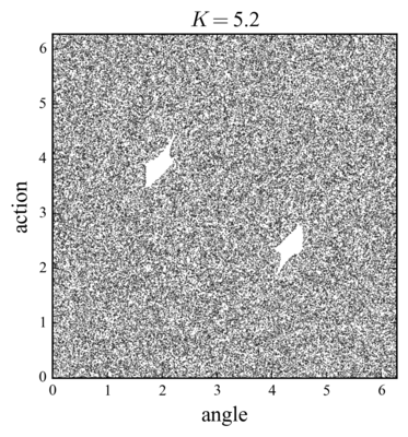
$$\lambda_\pm = \E^{\I a}, \quad \cos a = 1 - K/2\,, \; \sin a = \sqrt{K - K^2/4}\,,$$

and, nearby points on a circle around, are mapped to points in the same circle, hence $x=\pi$ is an elliptic point. In the case of the fixed point $x=0$, stable and unstable manifolds cross, and neighboring points are mapped along hyperbolas, that is, $x=0$ corresponds to a hyperbolic point. In fact, the elliptic point becomes a hyperbolic point at $K=4$. We can speculate that above this threshold the whole phase space becomes chaotic.

Exercice

Investigate the behavior of the standard map as a function of $K$

def standard_n(K, N):
    N0 = 20
    p = linspace(-pi, pi, N0)
    x = pi*ones(N0)
    #
    for n in range(N):
        p = mod(p + K*sin(x), 2*pi)
        x = mod(x + p, 2*pi)
        plot(x, p, 'k.', ms = 0.5, alpha=0.5)

The behavior near $K=4$ is interesting:

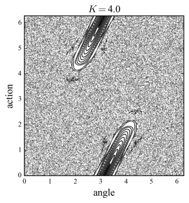
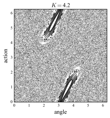
We observe the disappearance of the elliptic point and the formation of two separated islands within a stochastic sea.

»chaos »stability »hamiltonian systems »plasmas