»chaos »maps »stability »hamiltonian systems »quasilinear theory

$\newcommand{\I}{\mathrm{i}} \newcommand{\E}{\mathrm{e}} \newcommand{\D}{\mathop{}\!\mathrm{d}} \newcommand{\Di}[1]{\mathop{}\!\mathrm{d}#1\,} \newcommand{\Dd}[1]{\frac{\mathop{}\!\mathrm{d}}{\mathop{}\!\mathrm{d}#1}}$

Warm plamas and the Vlasov equation

A plasma is loosely defined as the fourth state of matter; it is basically an ionized gas whose physical properties depend on the electrostatic interaction between the charged particles. There is a large variety of plasma states depending on their characteristic densities and temperatures. Plasma density $n$ and temperature $T$ can cover a wide range of scales, from rarefied weakly ionized discharges to hot completely ionized plasmas as in a tokamak or in the solar corona.

The one particle distribution function in a $d$-dimensional phase space $(x,v)$,

\begin{equation} \label{fxv} f = f(x,v,t)\,, \quad \int_{-\infty}^{\infty} \Di{v} f(x,v,t) = n(x,t) \end{equation}

of an electron plasma [here $n=n(x,t)$ is the electron density] in a neutralizing background $n_0$ of positive charge, satisfies the Vlasov equation

\begin{equation} \label{vlasov} \frac{\partial f }{\partial t} + v \frac{\partial f}{\partial x} + \frac{e}{m} \nabla \varphi(x,t) \frac{\partial f}{\partial v} = 0\,, \quad -\nabla^2 \varphi(x,t) = \frac{e}{\epsilon_0} \left[ n_0 - \int_{-\infty}^{\infty} \Di{v} f(x,v,t) \right]\,. \end{equation}

The one particle dynamics is driven by the self-consistent electrostatic electric field $E=-\nabla \varphi$, where $\varphi = \varphi(x,t)$ is the potential. Indeed, the forces exerted on an individual charge are due, because of the long range of the Coulomb force, to the electric field $E$ created by all the other charges in the plasma. Vlasov equation is a mean field approximation that neglects two-body collisions. Note that among the physical parameters there is the electron mass $m$ and charge $-e$, which are relevant at the microscopic one particle scale; moreover, we also have a macroscopic parameter $n_0$, the density of the ions, supposed to be uniform. The presence together of the microscopic and macroscopic parameters reveals the nature of the Vlasov equation: it is a kinetic equation, relating the motion of individual particles with the thermodynamic state of the system.

Plasma waves

In a hot plasmas waves of many different kinds can propagate; in the simplest case, an electron plasma with uniform ion background, a fluctuation of the charge density gives rise to a longitudinal wave, the Langmuir or plasma wave. At thermodynamic equilibrium the plasma density is $n(x,t) = n_0$ is homogeneous and the velocity distribution is Maxwellian $f(x,v,t)=f_0(v)$:

$$ f_0(v) = n_0 (m/2\pi T)^{3/2} \E^{-m v^2/2T} $$

where we took the Boltzmann constant one.

We start studying the dimensions of the physical parameters

$e,\epsilon_0$ are purely dimension dependent constants, $m$ can be taken as the unit of mass, and $n_0,T$ characterize the thermodynamic state;
the units of mass, length and $(\text{time})^{-1}$ are given by monomial combinaisons of the dimensional parameters:

$$ m\,, \quad \lambda_D = \sqrt{\frac{\epsilon_0 T}{e^2 n_0}}\,, \quad \omega_p = \sqrt{\frac{e^2 n_0 }{\epsilon_0 m}}\,,$$

where $\lambda_D$ is the Debye length and $\omega_p$ the plasma frequency; $\lambda_D$ mesures the range of the Coulomb forces in a plasma and $\omega_p$ is a natural electrostatic oscillation frequency of the charge density;
from these parameters one can form the nondimensional plasma parameter

$$g=\frac{1}{\lambda_D^3 n}$$

which is the inverse of the ratio between the Debye length and the mean distance between particles uniformly distributed in space, or equivalently, it is inversely proportional to the number of particles in a sphere of $\lambda_D$ radius, inside which Coulomb interactions are important. Therefore, $g$ measures the strength of thermal forces with respect to Coulomb forces; it is small when collective effects are important (many particles within $\lambda_D$).

Exercice

Show, using simple fluid equations, that (i) the plasma frequency corresponds to charge density fluctuations, and that (ii) a test charge potential is screened at distances of the order of the Debye length.

In the following we use the above units to get nondimensional expressions. The different physical regimes of the collisionless unmagnetized electron plasma depend on the sole plasma $g$ parameter. We assume the hot, diluted, Coulomb interaction dominated regime, $g \ll 1$.

The linearized Vlasov equation reads, in Fourier space $(\omega,k)$:

$$ (-\I \omega + \I k \cdot v)f_{\omega k} = \I k \cdot \frac{\partial }{\partial v}f_0(v) \varphi_{\omega k} \,, \quad k^2 \varphi_{\omega k} = \int dv f_{\omega k}$$

from which one straightforwardly obtains the dispersion relation,

\begin{equation} \label{dispersion} \varepsilon(\omega,k) = 1 + \frac{1}{k^2} \int_{\mathrm{V}(v)} \Di{v} \frac{k\cdot \frac{\partial f_0}{\partial v} }{\omega -k\cdot v} \end{equation}

where $\mathrm{V}(v)$ is the volume in velocity space. Landau showed that the integral (which is devergent because of the resonance $\omega = k \cdot v$), must be extended to the $\omega \in \mathbb{C}$ plane:

\begin{equation} \frac{1}{\omega - k \cdot v + \I o} = \frac{\mathcal{P}}{\omega - k \cdot v} - \I \pi \delta(\omega - k \cdot v) \end{equation}

(Plemelj formula, in the limit $o \rightarrow 0$) with $\mathcal{P}$ denoting the principal value. The physical justification of this prescription is causality, $\omega$ must include a small positive imaginary part.

The real $\omega = \omega(k)$ solution of ($\ref{dispersion}$) corresponds to the Langmuir waves. The pole in the denominator only involves the component component $v$ of the velocity parallel to the wave vector $k$; therefore it is enough to take this one dimensional velocity direction and use the corresponding one dimensional Maxwell distribution. In the hydrodynamic limit $k \rightarrow 0$ we can expand the integrand in powers of $k$, to get after an integration by parts

\begin{equation} \mathcal{P} \int_{-\infty}^{\infty} \frac{ \Di{v} }{k} \frac{\frac{\partial F_0}{\partial v} }{\omega -kv} = \int_{-\infty}^{\infty} \Di{v} \frac{F_0(v)}{(\omega - kv)^2} \approx \frac{1}{\omega^2} \left( 1+ \frac{3k^2}{\omega^2} \right)\,, \end{equation}

where $F_0$ is the one dimensional Maxwell distribution (depending on the longitudinal velocity).Using this result in ($\ref{dispersion}$) we obtain the dispersion relation for the plasma waves:

\begin{equation} \omega(k) = 1 + \frac{3}{2}k^2 \quad \Rightarrow \quad \omega(k) = \omega_p + \frac{3}{2}(\lambda_D k)^2 \end{equation}

where, in the last equality, we put the dimensional parameters.

Landau damping

The imaginary part of the dispersion relation describes the damping (and in principle also the amplification) of the plasma waves. This gives rise to an imaginary part of the frequency $\gamma = \mathrm{Re}\,\omega$, which controls the long time behavior of the electric field $E \sim \E^{\gamma t}$; a negative $\gamma$ is then related to damping of the electrostatic fluctuations. This astonishing phenomenon in a system which is invariant under time reversal, and where any collisions can introduce dissipation, was discovered by Landau. In this case the integral is trivial and gives:

\begin{equation} \varepsilon(\omega,k) = 1- \frac{1}{ \omega^2} (1+ 3 \frac{k^2}{\omega^2} )- \frac{\I \pi }{k^2} \left. \frac{\partial F_0(v) }{\partial v} \right|_{v=\frac{\omega}{k} } = 0 \,, \quad \omega \in \mathbb{C}\,, \end{equation}

from which we finally find the imaginary part of the frequency,

\begin{equation} \gamma(k) = - \frac{ \mathrm{Im}\, \varepsilon(\omega,k) }{\displaystyle \frac{ \partial \mathrm{Re}\, \varepsilon(\omega,k) }{\partial \omega } } = \frac{\pi \omega^3}{2k^2} \left. \frac{\partial F_0(v) }{\partial v} \right|_{v=\frac{\omega}{k} } \end{equation}

in the same approximation $k \rightarrow 0$ and $\mathrm{Re}\, \omega \gg \mathrm{Im}\, \omega = \gamma$. For the Maxwellian it becomes,

\begin{equation} \gamma(k) = - \sqrt{\frac{\pi}{8}} \frac{1}{k^3} \exp \left[- \frac{1}{2 k^2}\right] \end{equation}

or in dimensional form

\begin{equation} \gamma(k) = - \sqrt{\frac{\pi}{8}} \frac{\omega_p}{(\lambda_D k)^3} \exp \left[- \frac{1}{2 (\lambda_D k)^2}\right]\,. \end{equation}

We observe that the sign of the Landau rate $\gamma$ depends on the slope of the distribution function at the wave phase space velocity $v=\omega/k$, and for the Maxwellian this slope is strictly negative, corresponding to a damping rate. In the opposite case, for example if a bump of rapid particles is present, a positive slope in the velocity distribution function appears, and the plasma is unstable.

Nonlinear evolution

The description of the evolution of an unstable plasma needs numerical methods. A difficulty for any numerical approach, is that the distribution function, even if initially smooth, mixing in phase space creates finer and finer structures. Therefore, discretisation grids are not well adapted. An interesting algorithm that avoids, at least in part, these difficulties is the so called particle in cell method. It is based on the fact that de distribution function is constant along the trajectories of “particles” (set of points in phase space):

\begin{equation} \dot{x_p} = v_p\,, \quad \dot{v_p} = - E(x) \end{equation}

with time measured un plasma frequencies, and $e=m=\epsilon_0=1$, $p$ is the particle index, and the electric field, which depends on the position of all the other particles, is computed from the Poisson equation,

\begin{equation} -\nabla^2 \phi(X) = 1 - \frac{n(X)}{n_0} \end{equation}

computed on a spatial grid $X$. The charge density $n(X)$ is constructed as a histogram of particle positions, using first order interpolation. We give here an example of a code (in python):

Computation of the density at a grid point $X[j]$ from the particles positions $x[p]$, $j$ is the spatial grid index:

# NP number of particles
# NX number of lattice points in x
# L length
# DX = L/NX
def density(x):
    """weithed histogram of particle positions"""
    n = zeros(NX)
    for p in range(NP):
        j = int(x[p]/DX)
        j1 = j + 1
        if j < NX - 1:
            n[j] += (X[j1] - x[p])/DX
            n[j1] += (x[p] - X[j])/DX
        # only j == NX -1 case
        else:
            n[j] += (L - x[p])/DX
            n[0] += (x[p] - X[j])/DX
    return 1 - n/N0

Computation of the force on particle $x[p]$; the first task is to solve Poisson equation using fast Fourier transforms, second, to compute the gradient of the potential to get the electric field, and finally, to interpolate the electric field on the grid, for each particle, the obtain the force:

# iLap ~ -1/k^2 is the inverse of the laplacian (k != 0)
# pseudo-spectral method
def force(x, n):
    """electric potential in X""" 
    pot = zeros(NX)
    fp = zeros(NX)
    #
    # solution of the Poisson equation
    pot = real( ifft( iLap * fft(n) ) )
    #
    # gradient
    fp = -(roll(pot,-1) - roll(pot,1))/(2*DX)
    #
    # force on particle p (interpolation)
    f = zeros(NP)
    for p in range(NP):
        j = int(x[p]/DX)  # j is < NX - 1
        j1 = j + 1
        if j < NX - 1:
            f[p] += fp[j]*(X[j1] - x[p])/DX + \
                    fp[j1]*(x[p] - X[j])/DX
        # only j == NX -1 case
        else:
            f[p] += fp[j]*(L - x[p])/DX + \
                    fp[0]*(x[p] - X[j])/DX
    return f

Leap-frog algorithm to time stepping:

# DT time step
# f the force applied at position x
def lf(x, v, f):
    """leap-frog time stepping"""
    v += -DT*f
    x += DT*v           
    return mod(x, L), v

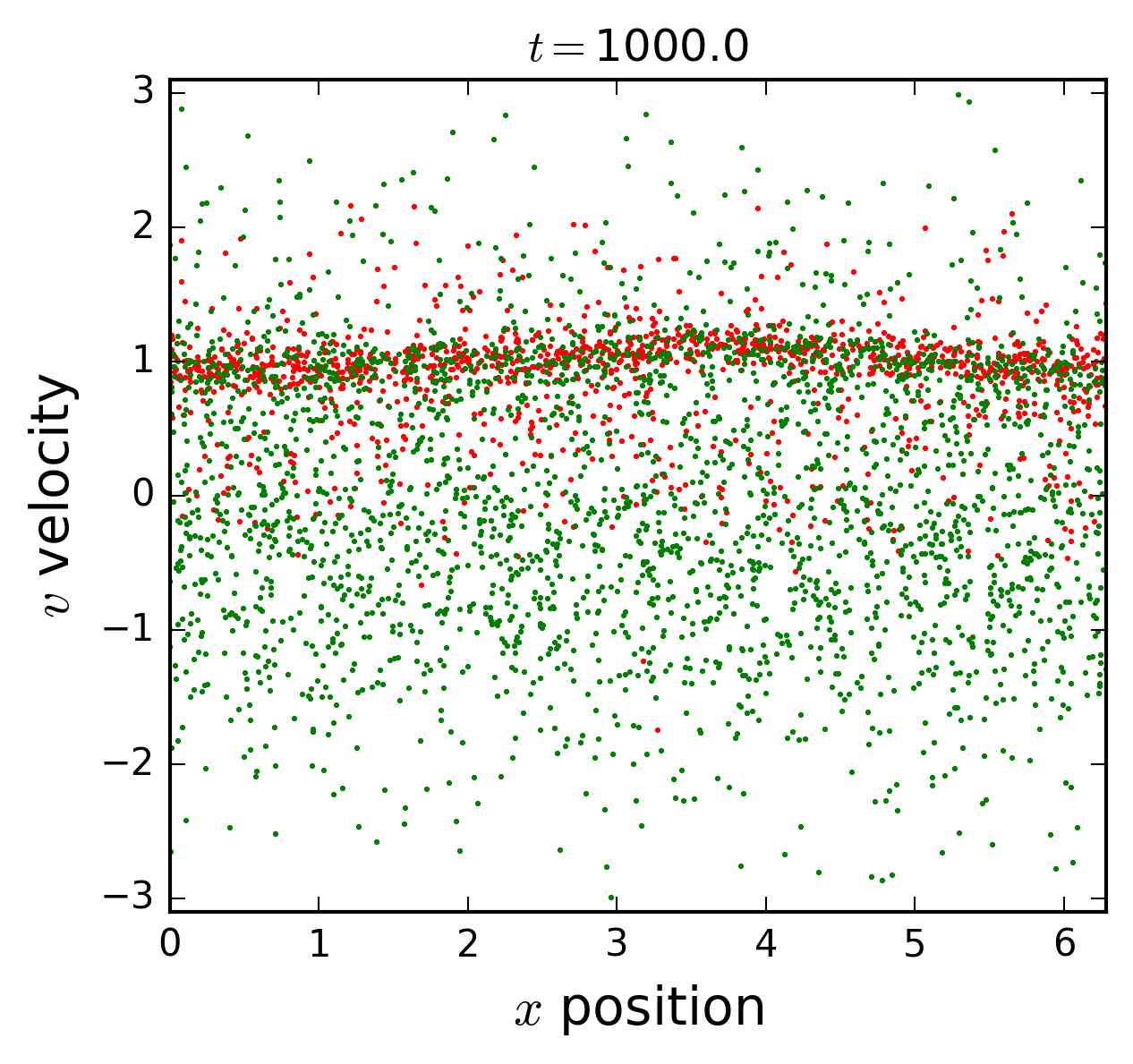
Two beams instability

In the initial state two uniform streams of electrons moving in opposite directions; a small perturbation of the density is introduced through a sinusoidal displacement of the equilibrium positions,

\begin{equation} x_p = x_{0p} + a \cos(k_0 x_{0p})\,, \end{equation}

where $a$ is the amplitude of mode $k_0=1$. In the figures we observe the wandering in phase space of the two streams, and the formation of a wide distribution in velocities.

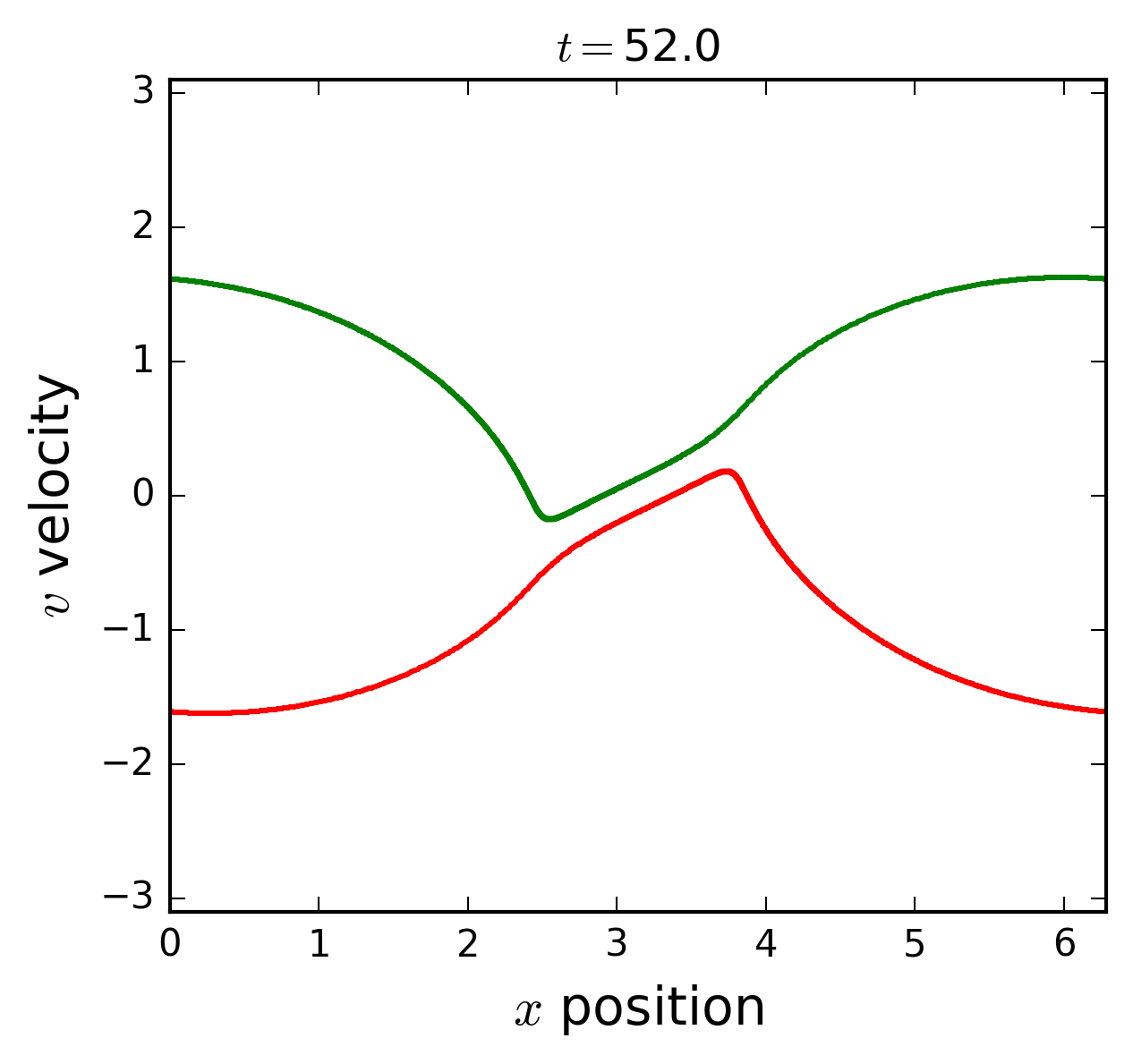
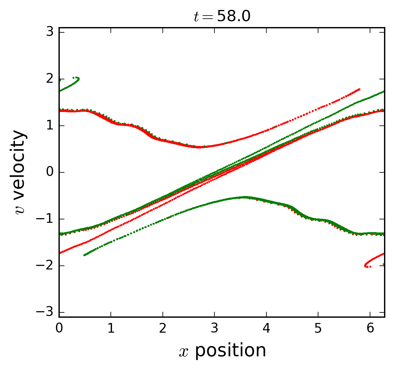
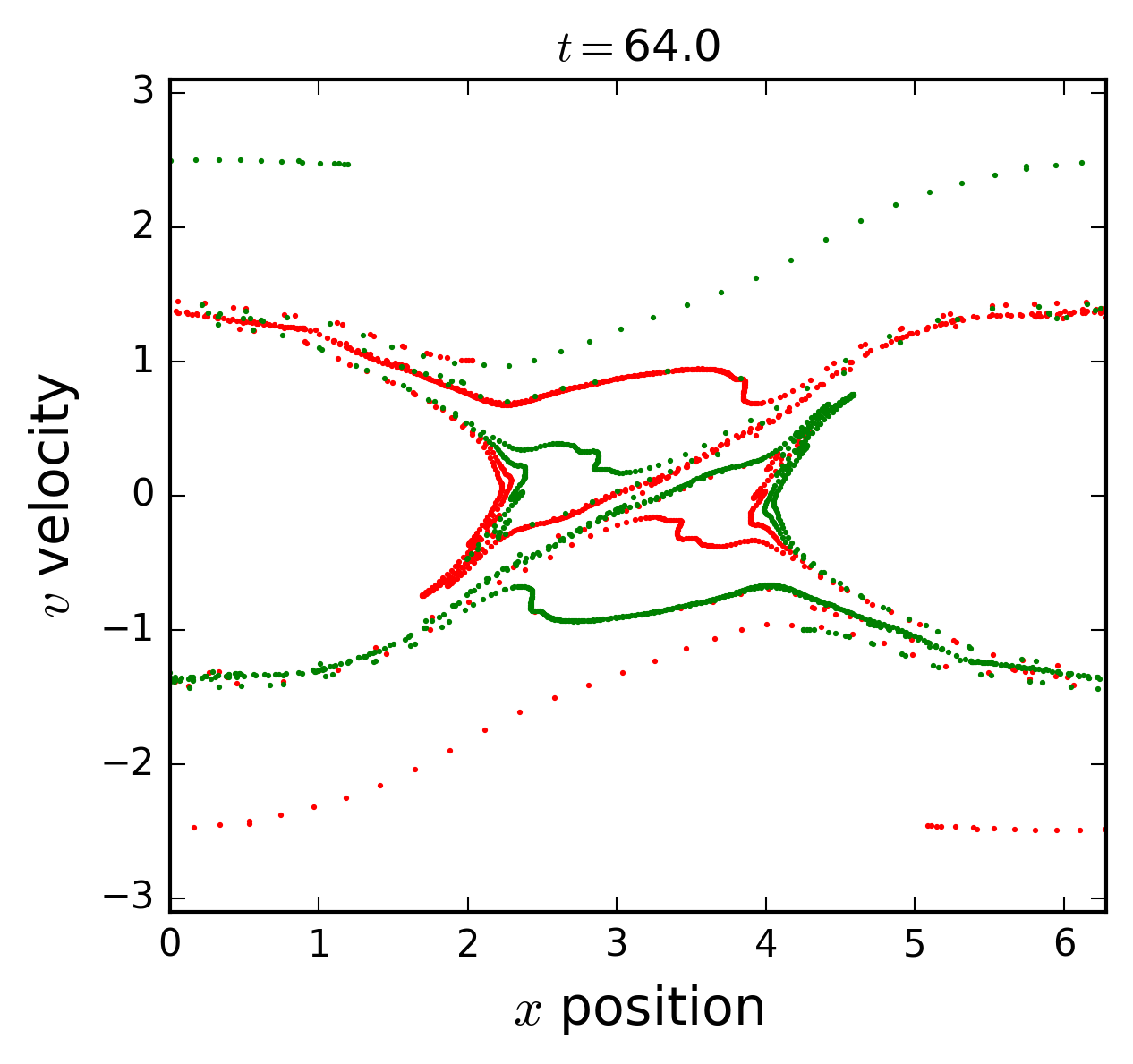
two beams 260 two beams 290 two beams 320

A notable characteristic of the distribution function is the formation of spiraling filamentary structures.

Exercise

Write a complete particle in cell code and investigate the bump on tail instability.

Bibliography

Kadomtsev Cooperative Effects in Plasmas, Springer, 2001. (.pdf)
Thorne and Blandford Modern Classical Phsycs, Princeton, 2017.
Boyd and Sanderson Plasma Physcis, Cambridge, 2003.
Bellan Fundamentals of Plasma Physics, Cambridge, 2008.

»chaos »maps »stability »hamiltonian systems »quasilinear theory