$\newcommand{\I}{\mathrm{i}} \newcommand{\E}{\mathrm{e}} \newcommand{\D}{\mathop{}\!\mathrm{d}} \newcommand{\Di}[1]{\mathop{}\!\mathrm{d}#1\,} \newcommand{\Dd}[1]{\frac{\mathop{}\!\mathrm{d}}{\mathop{}\!\mathrm{d}#1}}$

»quantum chaos »kicked rotator »dynamical localization »random matrices

Quantum walk

In a classical random walk the moving particle explores the configuration space at a rate growing as the square root of the number of steps $\sim \sqrt{t}$. Instead, a quantum walk, as first defined by Aharonov et al (1993), can explore its configuration space at much faster rate $\sim t$. This is a consequence of the superposition principle, at each time step, after the result of a coin toss, the moving particle initially at site $n$, simultaneously occupies the two neighboring sites with probabilities given by the square of the respective site amplitudes.

A step of a quantum walk is the result of the composition of two unitary operators, which gives an unitary evolution operator and a final measurement step:

Coin toss: coin tossing corresponds, in the simplest case, to a two state quantum system, $|\uparrow\rangle$ (up) and $|\downarrow>$ (down); commonly used coin $C$ operators are Hadamard $A$ and spin rotation $R$:
$$A = \frac{1}{\sqrt{2}} \begin{pmatrix} 1 & 1 \\ 1 & -1 \end{pmatrix} \,, \quad R(\theta) = \E^{-\I \sigma_y \theta/2} = \begin{pmatrix} \cos (\theta/2) & -\sin (\theta/2) \\ \sin (\theta/2) & \cos (\theta/2) \end{pmatrix}\,. $$
The action of both coin operators results in a superposition of the two up and down basis states, from an initial up or down state.
Shift: the motion step corresponds to the application of a shift operator (one step translation in the appropriated space), conditioned to the result of the coin tossing:

$$S=\sum_x \left( |x+1\rangle \langle x|\otimes |\uparrow\rangle\langle\uparrow| + |x-1\rangle \langle x|\otimes |\downarrow\rangle\langle\downarrow| \right)$$

where $\otimes$ denotes the Kronecker product; $S$ shifts the position $|x\rangle$ to the right $|x+1\rangle$, if the coin state is $|\uparrow\rangle$ or to the left $|x-1\rangle$, if it is $|\downarrow\rangle$.
Evolution: the walk dynamics is governed by the unitary operator,

$$U = S(I \otimes C)$$

that is the composition of $S$, a shift operator acting on a discrete space (position, energy, angular momentum states, etc.), and $C$ the coin operator acting on an internal degree of freedom; $I$ is the identity. Repeated application of $U$ leads to the history

$$|\psi_t\rangle = U^t |\psi_0\rangle$$

of the walker.
Measurement: the last step of the quantum walk algorithm consists in some projection to a specific state $|s\rangle$. The measure of $|s\rangle$ provides the probability of this state $|\langle s| \psi_t \rangle|^2$.

Exercice

Write a code to simulate the Hadamard random walk. Show that the evolution of a state initially at $x=0$ depends on the spin state: compare the sequences with initial coin states $|\uparrow\rangle$ and $(|\uparrow\rangle + \I |\downarrow\rangle)/\sqrt{2}$. Verify that $\langle x_t| x^2 |x_t\rangle\sim t^2$, where $|x_t\rangle$ is the state $|\psi_t\rangle$ projected to any coin state (summed over coin states), at time $t$ for large $t$.

Topology of the quantum walk

One of the goals of condensed matter physics is to characterize the different phases or states of matter: insulator, conductor, ferromagnetic, superfluid, etc. Landau establishes a theory that can account of these states and its changes, using the concept of order parameter, associated with the symmetries of the systems and the mechanisms that can brake these symmetries. A symmetry is broken, for instance, under the disorder-order transition, between a paramagnetic state and a ferromagnetic state when the temperature decreases. The isotropy of the magnetization field (the order parameter) in the paramagnetic state, is replaced by a magnetization directed along some specific direction, characteristic of the ferromagnetic state.

However, after the discovery of the quantum Hall effect, it became clear that other order states exists, not related to symmetries, but with the topology of, for instance, the electronic bands. Edge states in the integer and fractional Hall effect, solitons in one dimensional molecular chains (polyacetylene), or spin-polarized currents in topological insulators, are manifestations of some topological property of matter.

In order to identify the topology of a material, we use as an example the Bloch theory of electronic bands applied to a two dimensional material. We consider $|u_{\boldsymbol k}\rangle$, the Bloch function of quasi-momentum $\boldsymbol k$, and the system’s Hamiltonian $H(\boldsymbol k)$ which is a function of the quasi-momentum vector inside the Brillouin zone, $\boldsymbol k \in \mathrm{BZ}$. We assume that the material is an insulator whose energy bands, the set of eigenvalues of $H$, $E(\boldsymbol k)$, are separated by a gap. The topology of the band structure is related to the mapping from the crystal momentum space (the Brillouin zone), a torus in two dimensions, to the Hilbert space of the gapped Hamiltonian. If the gap remains open under changes of the quasi-momentum, the Hamiltonians belongs to the same topological class. These topological classes possess a Chern invariant $C \in \mathbb{Z}$, given by the (gauge independent) Berry flux integral:

\begin{equation} C = \frac{1}{2\pi} \oint \D^2 \boldsymbol k \cdot \boldsymbol F\,, \quad \boldsymbol F = \frac{\partial }{\partial \boldsymbol k} \wedge \boldsymbol A\,,\quad \boldsymbol A = -\I \langle u_{\boldsymbol k}| \frac{\partial }{\partial \boldsymbol k} |u_{\boldsymbol k}\rangle \end{equation}

where the Berry connexion $\boldsymbol A$ and the curvature $\boldsymbol F$ are the analogs of the vector potential and the magnetic field; this analogy comes from the indeterminate eigenvector’s phase $|u_{\boldsymbol k}\rangle \rightarrow \E^{\I \phi(\boldsymbol k)} |u_{\boldsymbol k}\rangle$, which translates into the gauge transformation $\boldsymbol A \rightarrow \boldsymbol A + \partial_{\boldsymbol k} \phi(\boldsymbol k)$. The Chern number itself, appears as the charge of a magnetic monopole, in this analogy.

Su Schrieffer Heeger model

The simplest non trivial topological system is a two-band model with hopping amplitudes between sites of type A and B:

\begin{equation} H = \sum_{x=1}^{L} (\epsilon + \Delta) c^\dagger_{\mathrm{A},x} c_{\mathrm{B},x} + \sum_{x=1}^{L-1} (\epsilon - \Delta) c^\dagger_{\mathrm{A},x+1} c_{\mathrm{B},x} + \text{hc}\,, \end{equation}

we take the length of the unit cell equal to one. This model was first introduced by Su, Schrieffer and Haager (1979) to investigate the charge transfer in polyacetylene, a (CH) chain with alternating double bonds. $H$ takes into account, in the tight binding approximation, the two kind of bonds $\epsilon + \Delta$ (double bond) in the unit cell (AB) and $\epsilon - \Delta$ (single bond) between cells. Two equivalent phases are possible by exchange of single and double bonds: for example a chain with an initial double bound (phase A) and other with an initial single bond (phase B); putting both together introduces a defect, two successive single bonds, for instance. Exchange of the bond pattern corresponds to a sign change of the parameter $\Delta$, which is also proportional to the energy gap between the two electronic bands $\Delta$.

Using a momentum representation $k$, and introducing a spinor $\psi_k$,

$$ \psi_k = \begin{pmatrix} a_k \\ b_k \end{pmatrix} \,, \quad a_k = \frac{1}{\sqrt{N}}\sum_n \E^{-\I x k} c_{\mathrm{A},x}\,, \quad b_k = \frac{1}{\sqrt{N}}\sum_n \E^{-\I x k} c_{\mathrm{B},x} $$

the Hamiltonian can be written in the diagonal form:

\begin{equation} H = \sum_k \psi^\dagger_k \boldsymbol d(k) \cdot \boldsymbol \sigma \psi_k \,,\quad d_x = (1 + \Delta) + (1 - \Delta) \cos k\,, \quad d_y = (1 - \Delta) \sin k \end{equation}

(taking $\epsilon=1$, the energy scale) from which we readily find the two eigenvalues

\begin{equation} E_\pm = \pm \sqrt{ d_x^2 + d_y^2} = \pm d \end{equation}

and the eigenvectors,

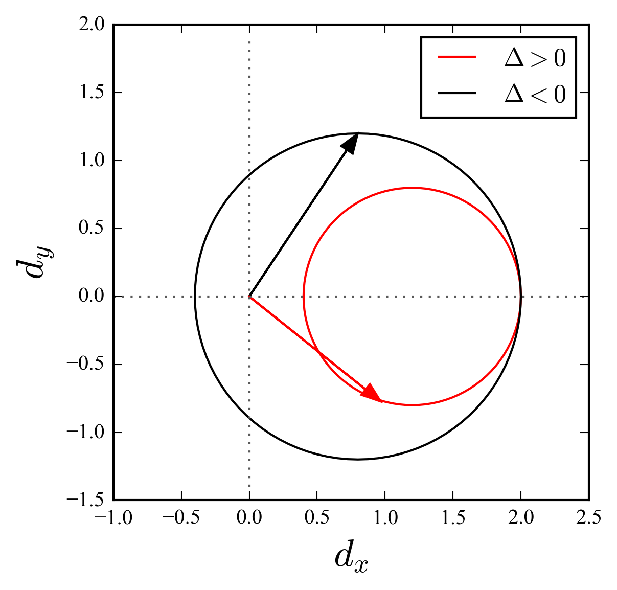
\begin{equation} u_+ = \frac{1}{\sqrt{2}} \begin{pmatrix} 1 \\ \E^{\I \varphi_k} \end{pmatrix}\,, \quad u_- = \frac{1}{\sqrt{2}} \begin{pmatrix} 1 \\ -\E^{\I \varphi_k} \end{pmatrix} \end{equation}

Varying the value of $k$ in the circle $(-\pi,\pi)$, the vector $\boldsymbol d(k)$ describes a circle; if $\Delta>0$ the circle do not contain the origin, but if $\Delta<0$ it will contain the origin. The winding number can be computed from the logarithm of the complex function $h(k) = d_x(k) - \I d_y(k)= |E_k|\exp[\I \mathrm{Arg}\,h(k)]$:

\begin{equation} C = \frac{\I}{2\pi}\int_{-\pi}^{\pi} \Di{k} \frac{\partial }{\partial k}\log q(k)\,, \quad q = \frac{h}{|h|}\,. \end{equation}

Using the above definitions, one gets

\begin{equation} C = \begin{cases} 0, &\text{ if } \Delta > 0 \\ 1, &\text{ if } \Delta < 0 \end{cases} %> \end{equation}

The rotation quantum walk

We consider a walker on a one dimensional lattice of points $x$, whose motion is determined by the orientation of its spin. A single step decomposes in:

a spin rotation $R(\theta) = \E^{-\I \sigma_y \theta}$,

$$R_y(\theta) = \begin{pmatrix} \cos\theta & -\sin\theta\\ \sin\theta & \cos\theta \end{pmatrix}$$
and a shift $S=S_\downarrow + S_\uparrow$ towards the left $S_\downarrow$ for the spin down, and to the right $S_\uparrow$ for the spin up,
the evolution operator is

$$U = S [I \otimes R(\theta)] \equiv \E^{-\I H_{\text{eff}}}$$

where we defined an effective Hamiltonian.

Using the momentum representation

$$S = \int_{-\pi}^{\pi} \Di{k} |k\rangle\langle k| \otimes \E^{\I k \sigma_z}$$

the effective Hamiltonian becomes diagonal

\begin{equation} H_{\text{eff}} = \int_{-\pi}^{\pi} \D k\, |k\rangle\langle k| \otimes E_\theta(k) \boldsymbol n_\theta(k) \cdot \boldsymbol \sigma \end{equation}

with the energy spectrum

\begin{equation} \cos E_\theta(k) = \cos \theta \cos k \end{equation}

and the spin quantization axis $\boldsymbol n_\theta(k)$ of the spinor eigenstates is,

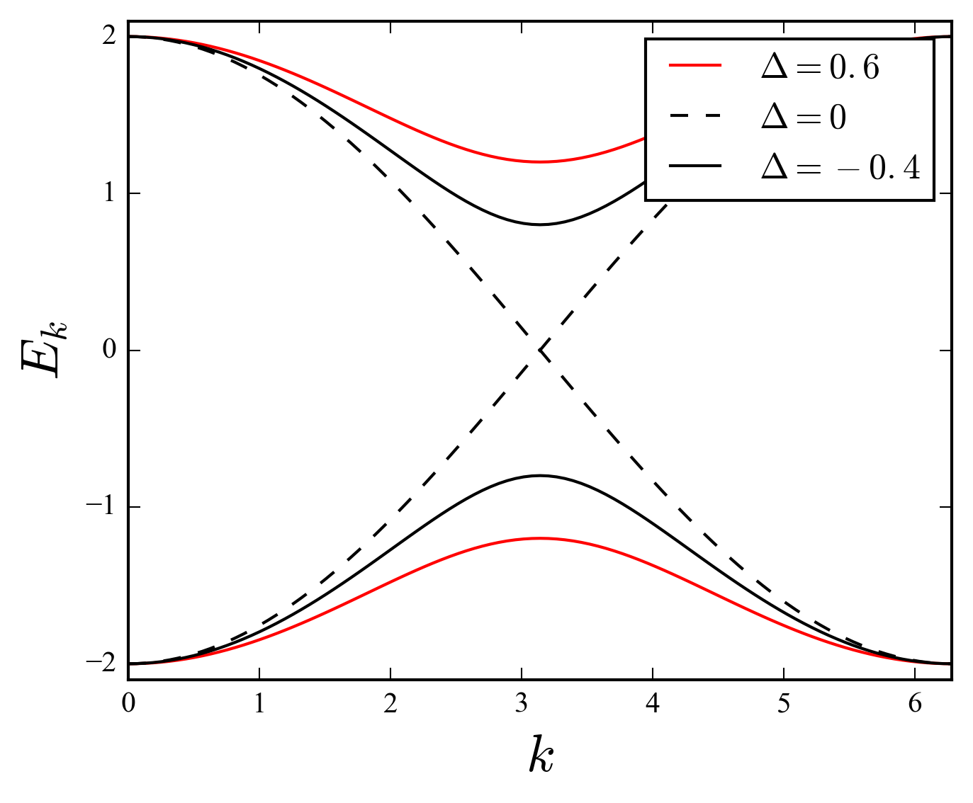
\begin{equation} \boldsymbol n_\theta(k) = \frac{1}{\sin E_\theta(k)} \begin{pmatrix} \sin \theta \sin k\\ \sin \theta \cos k\\ -\cos \theta \sin k \end{pmatrix} \end{equation}

The dispersion relation of the rotation quantum walk $E_\theta(k)$, for various values of $\theta=0,\pi/6,\pi/2,5\pi/6$; $\theta=0$ shows a dirac point at $k=0$; $\theta = \pi/2$ gives flat bands; intermediate values of $\theta$ show gapped bands. Observe de similarity with the polyacetylene model. Below and above the dirac point, the bands topology changes.

It is worth noting that at $\theta = 0, \pi$ the unit vector $\boldsymbol n$ has a singularity: numerator and denominator vanish at $k=0, \pi$. Geometrically, it corresponds to a discontinuity of the normal vector $\boldsymbol A(\theta)$, the unit vector perpendicular to the plane of rotation defined by $\boldsymbol n_\theta(k)$ when $k$ varies between $(-\pi,\pi]$:

$$\boldsymbol A(\theta) = -\mathrm{sgn}(\sin\theta) (\cos \theta, 0, \sin \theta)\,,$$

which can be obtained using, for instance, two points $k=0,\pi/2$ on the circle,

$$\boldsymbol A(\theta) = \frac{\boldsymbol n_\theta(0) \times \boldsymbol n_\theta(\pi/2)}{|\boldsymbol n_\theta(0) \times \boldsymbol n_\theta(\pi/2)|}\,.$$

The figure shows the rotation of the $\boldsymbol d_\theta(k)$ vector for $\theta=-\pi/8$ (black) and $\theta = \pi/8$: a discontinuous change of rotation occurs at $\theta=0$.

The vector $\boldsymbol A$ can be used to demonstrate the existence of a chiral symmetry associated with the effective hamiltionian:

$$\E^{\I \pi \boldsymbol A \cdot \boldsymbol \sigma/2} H \E^{-\I \pi \boldsymbol A \cdot \boldsymbol \sigma/2} = - H\,.$$

A change in the sigh of $\theta$ is accompanied with a chirality change: trying to put together the two walks, will create a “defect” as in the SSH model: an edge state with zero (op $\pi$) energy, spatially localized.

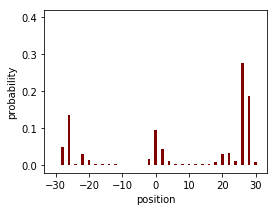
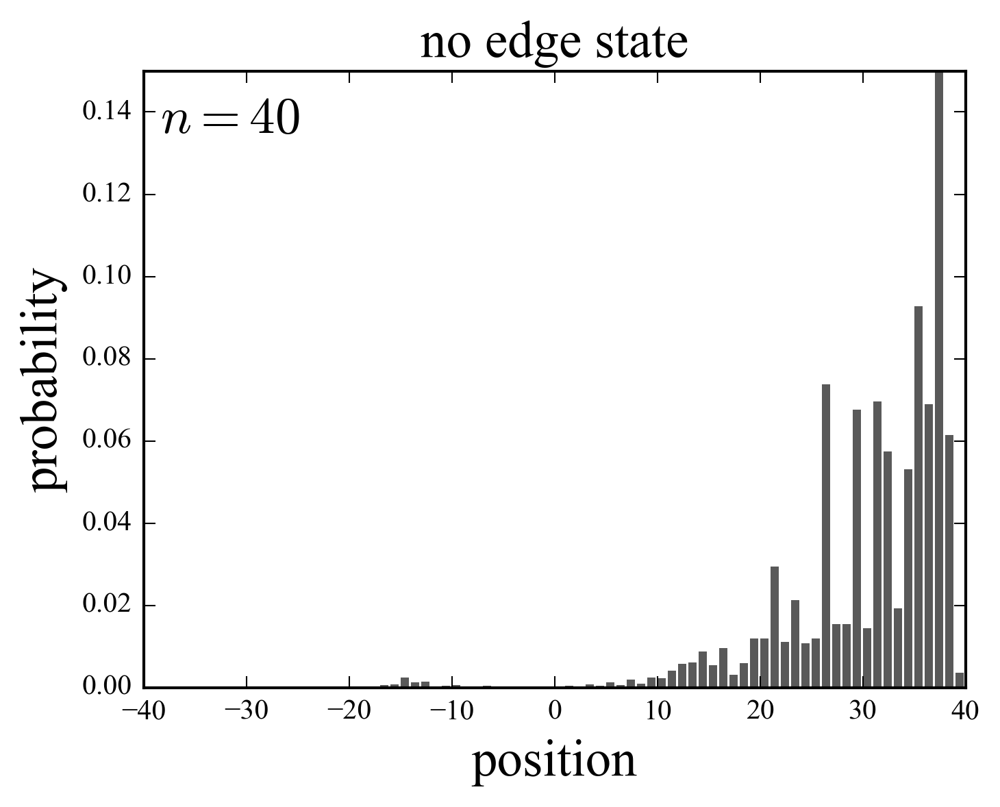
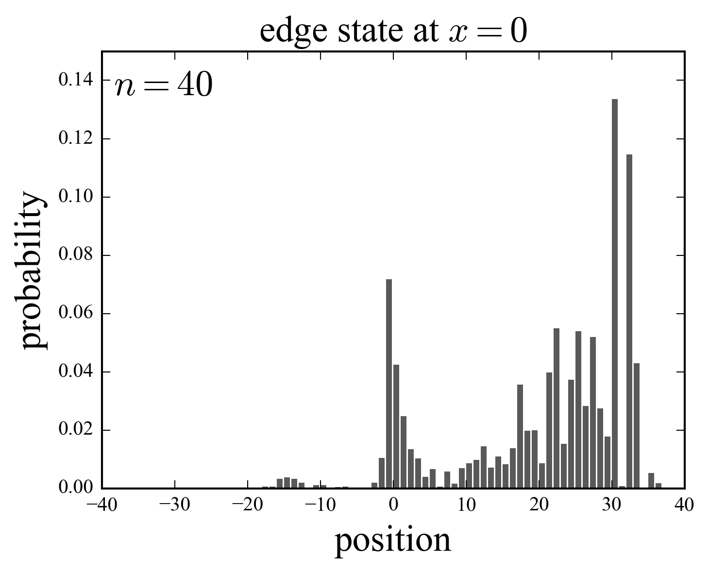
Using a python code we can investigate the behavior of the quantum walk when an interface separating two topologically different regions is introduced at $x=0$. The angle of rotation is split into two values $\theta_-$ on the left of the origin ($x\le0$) and $\theta_+$ on the right ($x>0$.

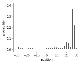
In the first figure the rotation angles on both sides of the interface are equal, and the normal ballistic propagation of the probability is observed. In the second figure a localized edge state appears at the interface separating, on the left, a $\theta<0$ region, and, on the right, a $\theta> 0$ region. One also observes the appearance of a reflected wave walking in the left direction.

Continuous limit

We investigate the low energy large wavelength behavior of the quantum walk by taking the hydrodynamic limit $E, k \rightarrow 0$. In this limit the effective hamiltonian,

$$H(\theta,k)= \frac{E_\theta(k)}{\sin E_\theta(k)} \begin{pmatrix} -\cos\theta \sin k & - \I \sin \theta \E^{\I k}\\ \I \sin \theta \E^{-\I k} & \cos \theta \sin k \end{pmatrix} $$

is given by,

$$H(\theta,k)= \tan\theta \sigma_y + \sec\theta (\sin \theta \sigma_x - \cos\theta \sigma_z) k$$

(to the lowest order in $k$). Making now the usual subtitution,

$$\I k \rightarrow \frac{\partial }{\partial x}$$

one obtains a Dirac—like hamiltonian

$$H_D = c \alpha p + m c^2 \beta$$

with speed term,

$$c = \frac{1}{\cos\theta},\quad \alpha = \cos\theta \sigma_x - \sin\theta \sigma_z$$

and mass term,

$$m c^2 = \tan\theta,\quad \beta = \sigma_y$$

We approximated

$$\frac{E \Delta t}{\sin( E \Delta t )} \approx \frac{1}{\cos\theta}$$

in order to preserve the property $|\boldsymbol n|^2=1$, or equivalently,

$$\alpha^2 = 1 ,\; \beta^2=1$$

where we put explicitly $\Delta t$ to show that the hydrodynamic limit is a two parameter approximation $E, k \rightarrow 0$, or $E\Delta t, k\Delta x \rightarrow 0$.

Simple quantum walk for three values of the rotation angle: $\theta = 0, \pi/2, \pi/4$. The initial state has probability one at $x=0$ and spin up. After 20 time steps the position probability is one at $x=20$ for $\theta = 0$, corresponding to a velocity $1$ and zero mass, thus the particle moves uniformly in the positive direction; for $\theta = \pi/2$, the mass and velocity become infinity, and the particle stays near its initial position. In fact, in this case the particle alternatively moves between $x=0$ and $x=1$. These results are in agreement with the prediction of the continuous limit. At intermediate values of $\theta$, the distribution is more complicated ($\theta=\pi/4$).

The split step walk

It is defined by the iteration of two simple steps with different angles:

$$U = S_-R_y(\theta_2)S_+R_y(\theta_1)$$

where $S_\pm$ move the up ($+$) and down ($-$) spins, respectively. A python implementation of the Kitagawa (2012) algorithm is as follows:

"""Reference: T. Kitagawa (2012) 
    "Topological phenomena in quantum walks",
    Quantum Information Processing vol. 11, p. 1107
"""
def rotation_1(N, theta):
    q = 0.5*theta*ones(2*N + 1)
    return array([[cos(q), -sin(q)], 
                  [sin(q), cos(q)]])

def rotation_2(N, theta_m, theta_p):
    x = arange(-N, N+1)
    delta = 0.01
    q = 0.5*((theta_p + theta_m)/2 + 
        (theta_p - theta_m)/2*tanh((x + 0.5)/delta))
    return array([[cos(q), -sin(q)], 
                [sin(q), cos(q)]])

def init_psi(N, a, b):
    psi = zeros((2, 2*N + 1))
    psi[0,N] = a
    psi[1,N] = b
    return psi

def mult(coin, psi):
    return einsum('ijk,jk->ik', coin, psi)

def qw_split(N, theta, theta_m, theta_p, a, b):
    r1 = rotation_1(N, theta)
    r2 = rotation_2(N, theta_m, theta_p)
    psi = init_psi(N, a, b)
    psi_t = zeros((2, 2*N + 1, N+1), dtype = complex)
    psi_t[:,:,0] = psi
    for n in range(1, N+1):
        #
        psi = mult(r1, psi) # rotation theta1
        psi[0] = roll(psi[0], 1) # shift up
        #
        psi = mult(r2, psi) # rotation theta2
        psi[1] = roll(psi[1], -1) # shift down
        #
        psi_t[:,:,n] = psi
    return psi_t

def measure(psi):
    return abs(psi[0,:])**2 + abs(psi[1,:])**2

Bibliography

János K. Asbóth, László Oroszlány, András Pályi, A Short Course on Topological Insulators: Band-structure topology and edge states in one and two dimensions, arXiv:1509.02295 [cond-mat.mes-hall] (.pdf).
Kempe J., Quantum Random Walks: An Introductory Overview, arXiv:quant-ph/0303081 (.pdf)
Kitagawa, T., Topological phenomena in quantum walks: elementary introduction to the physics of topological phases, Quantum Information Processes 11, 1107 (2012) (.pdf)

»quantum chaos »kicked rotator »dynamical localization »random matrices