$\newcommand{\I}{\mathrm{i}} \newcommand{\E}{\mathrm{e}} \newcommand{\D}{\mathop{}\!\mathrm{d}}$

»quantum chaos »kicked rotator »dynamical localization »quantum walk

Random matrices

Symmetry

We investigate the analog of classical canonical transformations, transformations preserving the hamiltonian structure in classical mechanics, to a quantum hamiltonian $H$. We are in particular interested in time reversal symmetry, which we use as a classifying criterion of different quantum systems.

Time reversal symmetry is, in quantum mechanics, associated with an antiunitary operator $\mathrm{T}$ such that it commutes with the hamiltonian and squares to one (integer spin) or minus one (half-integer spin):

$$[H,\mathrm{T}] = 0,\quad \mathrm{T}^2 = \pm 1\; .$$

As every antiunitary operator it can be written in terms of an unitary $U$ and the complex conjugation operator $\mathrm{K}$, $\mathrm{T} = U \mathrm{K}$. Its action renverses the sign of time, momentum, as ensured by the complex conjugation operator, and spin, as ensured by an unitary operator of spin rotation.

For a spinless particle $\mathrm{T} = \mathrm{K}$, as can be easily verified from the Schrödinger equation. For a spin $1/2$ particle a useful representation of the time reversal operator is

$$\mathrm{T} = \I\sigma_y \mathrm{K} = \E^{ \I \pi \sigma_y/2} \mathrm{K}\,.$$

General hamiltonians, unrestricted by antiunitary symmetries, belong to the unitary class. Indeed, a transformation

$$H\rightarrow AHA^{-1}$$

preserves the spectrum of $H$; imposing in addition that the transformed hamiltonian must also be hermitian leads to the condition of unitarity:

$$A^\dagger A = 1\,.$$

If the hamiltonian is time reversal symmetric with $\mathrm{T}^2=1$, it belongs to the orthogonal class, and can be written as a real matrix (operator):

$$H_{nm} = \langle n|H m\rangle = \langle \mathrm{T} n| \mathrm{T} H m\rangle^* = \langle \mathrm{T} n| \mathrm{T} H \mathrm{T}^2 m\rangle^* = \langle n|H m\rangle^* = H^*_{nm} $$

for a $\mathrm{T}$-invariant base $n,m,\ldots$, $\mathrm{T}|n\rangle=|n\rangle$.

When $\mathrm{T}^2=-1$, as in the one-half spin case, the energy levels are doubly degenerate (Kramers’ degeneracy): if $|n\rangle$ is an eigenstate of the hamiltonian then $|\mathrm{T} n\rangle$ is also an eigenstate, orthogonal to $|n\rangle$:

$$\langle n|\mathrm{T}n\rangle = \langle \mathrm{T} n|\mathrm{T}^2 n\rangle^* = -\langle \mathrm{T} n| n\rangle^* = -\langle n|\mathrm{T}n\rangle = 0\,.$$

In this case (without supplementary symmetries), a convenient basis of $H$ is given by $|1\rangle, \mathrm{T} |1\rangle,\ldots$. Therefore, the hamiltonian matrix can be decomposed in blocks of the form:

$$ h_{nm} = \begin{pmatrix} \langle n|H| m \rangle & \langle n|H| \mathrm{T} m \rangle\\ \langle \mathrm{T} n|H| m \rangle & \langle \mathrm{T} n|H| \mathrm{T} m \rangle \end{pmatrix}\,. $$

The time reversal operator can be written as $\mathrm{T} = \Omega \mathrm{K}$, where

$$ \Omega_{nn} = \begin{pmatrix} 0 & -1\\ 1 & 0\end{pmatrix}\,,\quad \Omega_{nm} = 0\,,\; n \ne m\,,$$

using the fact that

$$ |\psi\rangle = a|1\rangle + b|T1\rangle \rightarrow |\mathrm{T} \psi\rangle = a^*|\mathrm{T} 1\rangle - b^*|1\rangle \,.$$

Applying this to $H = \mathrm{T} H \mathrm{T}$ one obtains that the block $h$ is of the form:

$$h = a \tau_0 + \boldsymbol{b}\cdot \boldsymbol{\tau}, \quad \text{with}\; a, \boldsymbol{b}\in \mathbb{R},$$

where $\boldsymbol{\tau} = -\I \boldsymbol{\sigma}$ are antihermitian matrices ($h$ can be represented by a quaternion number).

Hamiltonians whose elements are quaternions belong to the symplectic class. A matrix $S$ that preserves the structure of the hamiltonian base $|1\rangle,|\mathrm{T} 1\rangle,\ldots$, so $S\Omega S^T = \Omega$, is a symplectic matrix; such a matrix commutes with the time reversal operator: $\mathrm{T} = S \mathrm{T} S^{-1}$:

$$S \mathrm{T} S^{-1} = S\Omega \mathrm{K} S^{-1} = S \Omega S^T \mathrm{K}= \Omega K\,.$$

In summary, according to its properties with respect to time reversal, we identified three board hamiltonian classes:

Unitary class, for systems without time reversal symmetry
Orthogonal class, for real hamiltonians, invariant with respect to time reversal with $\mathrm{T}^2=1$
Symplectic class, for time reversal symmetric hamiltonians with $\mathrm{T}^2 = -1$.

By considering other symmetries, say chiral or particle-hole that are important, for instance, in superconductors and topological insulators, more classes can be identified, see the review by Chiu et al. (2016) (arXiv .pdf).

Level repulsion

The symmetry class of the hamiltonian, orthogonal, unitary or symplectic, reflects in its spectral properties through the behavior of level crossings. Indeed, the number of parameters to specify the hamiltonian matrix, one real (orthogonal class), one complex (two reals, for the unitary class), and one quaternion (four reals, for the symplectic class), is related to the degree of level repulsion: an experimentally observable feature of the spectrum. From elementary quantum mechanics we know that integrable systems often show a high degree of degeneracy; for instance the hydrogen atom in a magnetic field shows levels crossing of Zeeman multiplets for increasing magnetic field. In general the behavior of levels as a function of a parameter on which the hamiltonian depends, it is different for a completely integrable case and for a generic case.

Consider the simplest two dimensional Hilbert space with one degenerate energy level $E_0$ perturbed by a potential $V$ of strength $|\lambda|$

$$H=\begin{pmatrix}E_0 & \lambda V \\ \lambda^* V^* & E_0\end{pmatrix}\,, \quad E_\pm = E_0 \pm |\lambda V|$$

for the orthogonal class, the single condition $\lambda = 0$ suffices to restore the degeneracy; for the unitary case two conditions are instead necessary $\mathrm{Re}\,\lambda = \mathrm{Im}\,\lambda = 0$. The degree $\beta$ of level repulsion is said to be $\beta=1$ and $\beta=2$ for the orthogonal and unitary classes, respectively. A similar reasoning shows that $\beta=4$ for the symplectic class.

As a consequence of level repulsion, the probability P(s) to find a vanishing spacing $s$ between two levels must tend to zero:

$$P(s) \sim s^\beta\,,\quad s\rightarrow0\,.$$

To see this, consider two neighboring levels of a generic hamiltonian (in the orthogonal class, to be specific), near the crossing we have,

$$H \sim E_0 \begin{pmatrix}x & y \\ y & -x\end{pmatrix}\,,\quad E_\pm = \pm E_0 \sqrt{x^2 + y^2}\,,$$

where both parameters $x,y$ are small; the two eigenvalues $E_\pm$ can be represented, as a function of the two parameters $x,y$, as a cone in the three dimensional space $(x,y,E)$. This is what is called a diabolic point. For the whole hamiltonian we have a set of crossings with a joint probability $W=W(x,y)$. The spacing distribution (in units of the mean spacing) is thus given by

$$p(s) = \int \D x \D y\, W(x,y) \delta\left(s - \Delta E(x,y)\right)\,.$$

where $\Delta E = (E_+ - E_-)/2E_0$ is the normalized energy gap. After a change of variables $\boldsymbol x \rightarrow s\boldsymbol x$ we obtain,

$$p(s) = s \int \D x \D y\, W(sx,sy) \delta\left(1 - \sqrt{x^2+y^2}\right) \sim s^\beta,\;\beta=1\,,$$

the probability goes linearly to zero for vanishing spacing (provided that $W(0)\ne 0)$. The value of the exponent is related to the dimension $d$ of the diabolic point, $\beta = d-1$; $d=3,5$ for the unitary and symplectic classes.

Gaussian ensembles

The statistical ensembles of hamiltonian matrices, supposed to describe the discrete spectrum of complex quantum systems, can be determined from a minimal set of hypothesis:

The elements $H_{nm}$ are identically distributed with probability $p(H_{nm})$
The symmetries of the hamiltonian are respected: for instance, the elements of the orthogonal class are real and the matrix symmetric.
A change of basis do not change the statistical properties of the ensemble. Therefore we must have, for the orthogonal class

$$P(H) = P(OHO^T)$$

where $O$ is an orthogonal matrix; and similarly for the other classes: the probability must be invariant under canonical transformations.

The third condition means that $P(H)$ must be a function of invariants like the trace $\mathrm{Tr} \, H$, and the determinant $\det(H)$. These assumptions are enough to show that

\begin{equation} \label{e1} P(H) = C \E^{-A \mathrm{Tr}\,H^2}\,, \end{equation}

the probability distribution of the hamiltonian matrices is gaussian ($A,C$ are constants).

To illustrate this result we consider the case of a $2\times2$ matrix in the $O(2)$ class. We want to compute

$$P(H) = p(H_{11}) p(H_{22}) p(H_{12})= p_1 p_2 p_{12} = P(OHO^T) = P(H')\,,$$

where the orthogonal (rotation) matrix has the form,

$$O(\theta) = 1 + \begin{pmatrix} 0 & -\theta \\ \theta & 0 \end{pmatrix}$$

(near the identity). The transformed hamiltonian is (to first order in $\theta$)

$$ H'_{11} = H_{11} - 2\theta H_{12} \;\rightarrow\; p'_1 = p_1 - 2 \theta H_{12} \frac{\D p_{1}}{\D H_{11}}$$

and analogously for $p'_2$ and $p'_{12}$. The invariance condition becomes,

$$ 0= \frac{1}{H_{12}} \frac{\D \ln p_{12}}{\D H_{12}} - \frac{2}{H_{11}-H_{22}} \left(\frac{\D \ln p_{1}}{\D H_{11}} -\frac{\D \ln p_{2}}{\D H_{22}}\right) $$

whose solution can be obtained using

$$ \frac{1}{H_{nm}} \frac{\D \ln p_{nm}}{\D H_{nm}} = \text{const.} $$

which immediately gives $p(H_{nm}) = a \exp(-b H_{nm}^2+cH_{nm})$, leading to the gaussian distribution $\eqref{e1}$ (choosing a zero of energy such that $H_{11}+H_{22} = 0$).

Level spacing distribution

As a straightforward application, we consider the level spacing distribution $p(s)$, using the same $2\times2$ approximation. If $\Delta E$ is the energy difference between two consecutive levels, the normalized spacing $s \sim \Delta E$ is defined so that its mean is one:

$$\int_0^\infty \D s \, p(s) = 1,\quad \int_0^\infty \D s \,s p(s) = 1\,.$$

The eigenvalues of the hamiltonian read,

$$E_\pm = \frac{H_{11}+H_{22}}{2} \pm \frac{1}{2} \sqrt{(H_{11}-H_{22})^2 + H_{12}^2}$$

In the diagonal base, obtained by a rotation of angle $\theta \rightarrow O(\theta)$,

$$H = O \,\mathrm{diag}H\,O^T,\quad O = \begin{pmatrix} \cos \theta & - \sin \theta \\ \sin \theta & \cos \theta \end{pmatrix}$$

we have,

\begin{align*} H_{11} &= E_+ \cos^2 \theta + E_- \sin^2 \theta \\ H_{22} &= E_+ \sin^2 \theta + E_- \cos^2 \theta \\ H_{12} &= (E_+ - E_-) \cos \theta \sin \theta \end{align*}

from which we can easily compute the jacobian:

$$ p(E_+,E_-,\theta) = P(H) \left| \frac{\partial(H_{11},H_{22},H_{12})}{\partial (E_+,E_-,\theta)} \right| = C |E_+-E_-| \E^{-A(E_+^2 + E_-^2)} $$

Taking $E_+ + E_- = 2 E_0$ and $E_+ - E_- = 2 D s$ (where $D$ is to be determined by imposing $\langle s\rangle = 1$), substituting these values into $p(E_+,E_-) = p(E_+(s, E_0), E_-(s, E_0))$, and using the normalization of $p(s)$, we finally obtain,

$$p(s) = \frac{\pi s}{2} \E^{-\pi s^2/4}\,.$$

This formula is known as the Wigner surmise; it is a remarkably good approximation for the general $N\rightarrow\infty$ case (figure and code below).

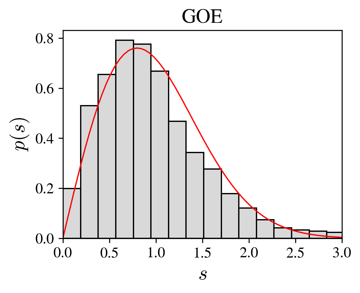
Wigner surmise (red line) and histogram of a single large matrix.

"""Compute the level spacings of a matrix in the GOE"""
n = 5000 # matrix size
g = random.normal(0,1,(n,n)) # nxn gaussian numbers
h = (g + g.T)/2 # real symmetric
e = eigvalsh(h) # eigenvalues
e = sort(real(e))
s = diff(e)/mean(diff(e)) # level spacings

The level spacings probability distribution is more generally obtained from the integral,

$$p(s) = C \int_{-\infty}^\infty \D E_+ \D E_-\, |E_+ - E_-|^\beta \E^{-A(E_+^2 + E_-^2)}\,\delta(s - |E_+ - E_-|)$$

which gives, for the unitary and symplectic classes the formulas

$$p(s) = \frac{32 s^2}{\pi^2} \E^{-4 s^2/\pi} $$

and

$$p(s) = \frac{2^{18} s^3}{3^6 \pi^3} \E^{-64 s^2/9\pi} \,,$$

respectively. For the “integrable” case, when the distribution of spacings is not restricted by repulsion, one has the Poisson distribution:

$$p(s) = \E^{-s}\,.$$

Exercices

Compare the Wigner surmise with numerical simulations of the three gaussian ensembles
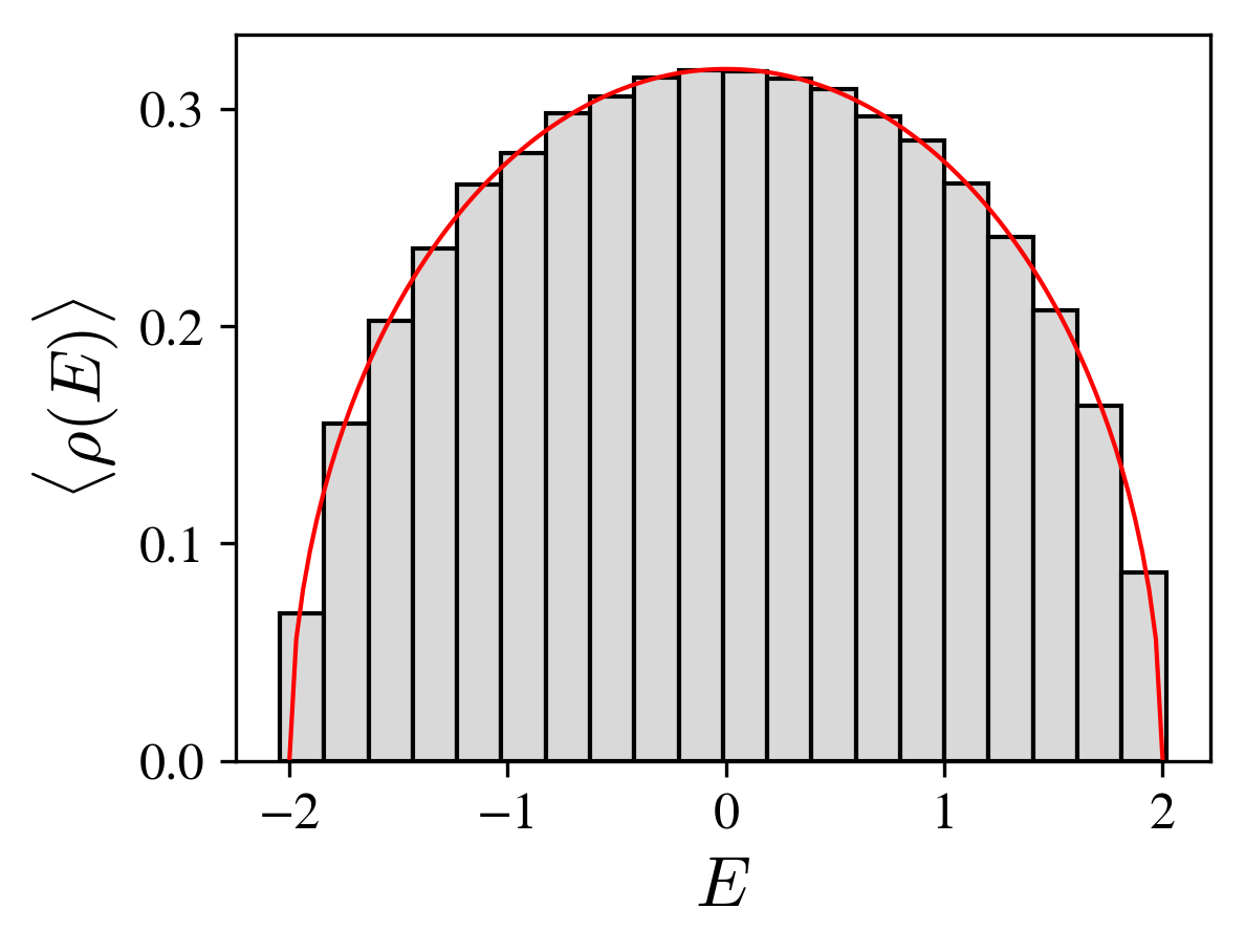
Show that the average distribution of energy levels for the gaussian orthogonal ensemble satisfies the Wigner semicircle law:

$$\langle \rho(E) \rangle = \frac{1}{2\pi} \sqrt{4 - E^2}$$

where $E$ is the normalized energy.
Investigate the distribution of the largest eigenvalue $\lambda = E_{\text{max}}$, of a hamiltonian matrix in the gaussian unitary ensemble, and verify that it follows the Tracy-Widom law $F_2$:

$$ F_2(\lambda) = \frac{\D}{\D \lambda}\exp\left[ -\int_{\lambda}^\infty \D t\, (t-\lambda) q(t)^2 \right] $$

where $q(t)$ is a solution of the Painlevé II differential equation

$$\ddot q(t) = t q(t) + 2 q(t)^3 $$

with the asymptote $q(t) \rightarrow \mathrm{Ai}(t)$ as $t \rightarrow \infty$, the Airy function. See Edelman et al. (2014) (.pdf)

Energy level distribution: the semicircle law

We consider the energy eigenvalues of a large $N$ hamiltonian matrix $H$ in the gaussian orthogonal ensemble. It is reasonable to think, by analogy with the Brownian motion, that the variance of $H$ increase with $N$, or equivalently that each matrix element is of order, $H_{nm}\sim \sqrt{N}$. Therefore, taking the constant $A$ in the probability distribution as $A \sim N$, ensures that the matrix elements are order one: $H/\sqrt{N} \sim \mathcal{O}(1)$. The gaussian orthogonal ensemble probability, after a simple rescaling of the hamiltonian, is then conveniently written as,

$$P(H) = c_N \exp\left[-\frac{N}{4}\mathrm{Tr}\,H^2\right]\,, \quad c_N = \frac{1}{2^{N/2}} \left( \frac{N}{2\pi} \right)^{N(N+1)/4}$$

where $N(N+1)/2$ is the number of independent elements of $H$; we also used

$$\mathrm{Tr}\,H^2 = \sum_n H_{nn}^2 + 2 \sum_{nm} H_{nm}^2\,.$$

We are interested in the statistical properties of the eigenvalues of $H$. The simplest quantity characterizing the distribution of energy levels is the density of states, defined by:

$$\langle\rho(E)\rangle = \frac{1}{N} \sum_{n=1}^N \langle\delta(E - E_n\rangle)\,,$$

where the angle brackets are for the averaging over the gaussian ensemble. We compute this quantity using its representation by a green function, and the replica method (see the references at the end of this section). We will demonstrate the Wigner semicircle law, as shown in the figure below (see also the exercise in the preceding section).

Wigner semicircle law

The retarded green function is defined by

$$G^R(E) = \frac{1}{E + \I o - H}$$

where $\I o \rightarrow 0$ ensures the convergence of the time dependent green function (fourier transform of $G^R(E)$) for past times ($t\rightarrow -\infty$). The retarded green function is analytic in the upper-half complex energy plane. The trace of the green function can be split into real and imaginary parts using the Plemelj formula

$$\mathrm{Tr}\, G^R(E) = \sum_n \frac{1}{E + \I o - E_n} = \sum_n \frac{\mathcal{P}}{E - E_n} - \I \pi \delta(E - E_na\,.)$$

Comparing this formula with the definition of the density of states, we obtain,

$$\langle \rho(E) \rangle = \frac{-1}{\pi N} \mathrm{Im} \mathrm{Tr}\,G^R(E)\,.$$

The trace of the green function can be written in terms of a determinant,

$$\mathrm{Tr}\, G^R(E) = \sum_n \frac{1}{E + \I o - E_n} = \frac{\partial }{\partial E} \sum_n \ln(E + \I o - E_n) = \frac{\partial }{\partial E} \ln \det(E + \I o - H)$$

Using this expression, we arrive at a formula of the averaged density of states,

$$\langle \rho(E) \rangle = \frac{-1}{\pi N} \mathrm{Im} \frac{\partial }{\partial E} \langle \ln \det(E + \I o - H)\rangle$$

whose computation reduces to the computation of the logarithm of a determinant. Now, to compute the determinant of a symmetric real matrix $A=A^T$, we can use its gaussian integral representation,

$$\frac{1}{(\det A)^{1/2}} = \int \D [x] \E^{-\frac{1}{2} x^T A x},\quad \D [x] = \prod_{n=1}^N \frac{\D x_n}{\sqrt{2\pi}}$$

where $x^T = (x_1 x_2 \ldots x_N)$ is a row vector. Once the determinant known it would remain the calculation of the mean of the logarithm over the random distribution of energies. A method to compute this averaging is to replace the logarithm by a simple power, using the elementary relation

$$\ln Z = \lim_{R\rightarrow0} \frac{Z^R-1}{R} = \left.\frac{\partial }{\partial R}\right|_{R=0} \, Z^R\,.$$

Therefore $\langle \ln Z \rangle \rightarrow \langle Z^R \rangle$, averaging of the logarithm becomes averaging over $R$ replicas of the original system (here described by $Z$). From this formula, defining

$$Z=[\det (E^+ -H)]^{-1/2}\,,$$

($E^+= E + \I o$) we finally obtain a suitable relation to compute the density of states averaged over the gaussian probability:

$$\langle \rho(E) \rangle = \frac{2}{\pi N} \mathrm{Im} \left.\frac{\partial} {\partial R}\right|_{R=0} \, \frac{\partial }{\partial E}\langle Z^R \rangle\,.$$

The explicit form of the determinant, incorporating the probability distribution of the hamiltonian matrix, is,

$$\langle Z^R \rangle = \int \prod_{r=1}^R \D[x_r] \int \D[H]\, \E^{-\frac{N}{4}\mathrm{Tr}\,H^2} \E^{-\frac{1}{2}\sum_{r=1}^R x^T_r (E^+ - H) x_r}$$

where

$$\D[H] = c_N \prod_{n,m}^N \D H_{nm}\,,$$

includes the probability normalization constant $c_N$. The gaussian integration is readily performed (completing the square, as usual):

$$\langle Z^R \rangle = \int \prod_{r=1}^R \D[x_r]\, \exp\left[- \frac{E^+}{2} \sum_{r=1}^R x^T_r x_r + \frac{1}{4N} \sum_{r,s=1}^R x^T_r x_r x^T_s x_s \right]$$

The fourth order term can be transformed into a second order term coupled to a $R\times R$ matrix $Q$ in the replica space,

$$\exp\left[ \frac{1}{4N} \sum_{r,s=1}^R x^T_r x_r x^T_s x_s \right] = \int \D[Q] \exp\left[ -\frac{N}{4} \mathrm{Tr}\,Q^2 \right] \exp\left[ \frac{1}{2} \sum_{r,s=1}^R x^T_r Q_{rs} x_s \right]\,,$$

this transformation leads to a gaussian integral over the vector $x$,

$$\langle Z^R \rangle = \int \D[Q] \E^{ -\frac{N}{4} \mathrm{Tr}\,Q^2 } \int \prod_{r=1}^R \D[x_r]\, \exp\left[- \frac{1}{2} \sum_{rs=1}^R x^T_r (E^+ \delta_{rs} - Q_{rs} ) x_s \right] $$

that can be readily evaluated, giving

$$\langle Z^R \rangle = \int \D[Q] \, \exp\left[-\frac{N}{4} \mathrm{Tr}\,Q^2 - \frac{N}{2} \mathrm{Tr}\, \ln (E^+\mathbb{1}_R - Q)\right] $$

Up to now all these formal calculations were exact: we transformed the original problem into an integral over replica matrices. The exponent of such integral contains a large parameter $N$, suggesting that the saddle point will give a solution in the limit $N \rightarrow \infty$. In addition, we also must calculate the limit of the replica parameter $R \rightarrow 0$, a kind of analytical continuation. Now, the first term in the exponential contains a diagonal term with $R$ terms, and a non-diagonal term with $R^2$ terms; the second term also contains $R$ terms. Therefore, we can assume that in the limit of $N \rightarrow \infty$ and small $R$, only the diagonal terms contribute to the saddle point:

$$Q_{rs} = q \delta_{rs}$$

this is the so-called replica symmetric ansatz, and in the present case it leads to the correct result. However, if we wanted to know the fluctuations at finite $N$, the replica symmetric assumption is no longer valid, and a more complete account of all the saddle points must be taken. Using the previous ansatz we have,

$$\langle Z^R \rangle \approx \left[ \int_{-\infty}^\infty \D q\, \E^{-\frac{N}{2}g(E,q)} \right]^R \approx \exp\left[ -\frac{NR}{2}g(E,q_*) \right]$$

where we neglected prefactor terms (subdominant), and $q_* = q_*(E)$ is the saddle point value of the exponent

$$g(E,q) = \frac{q^2}{2} + \ln(E^+ - q)\,.$$

For large values of $N$ the integral is dominated by the saddles in the complex $q$ plane of the exponent function $g(q)$. These saddle points are obtained from the condition $g'(q_*) = 0$,

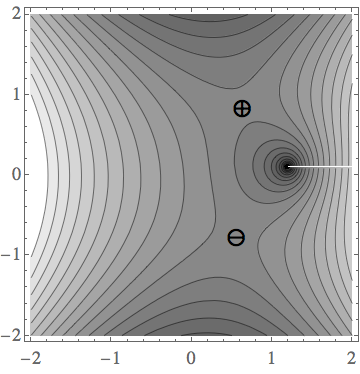
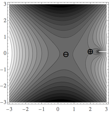
$$q - \frac{1}{E^+ - q} = 0, \quad q_\pm = \frac{E^+}{2} \pm \frac{1}{2} \sqrt{E^{+2}-4}$$

The figures below show the saddles for $E^+=1.2+\I 0.1$ (left) and $E^+=2.5+\I 0.1$ (right), of the function $\mathrm{Re}\, g(E^+,q)$ in the complex $q$ plane. For $|E|<2$, the pole at $q=E$ is shifted towards the upper half-plane by the positive small imaginary part of the energy; therefore, we can follow a path from $q\rightarrow-\infty$ to $q\rightarrow+\infty$ through the saddle $q_-$, along the lower half-plane. The other saddle, $q_+$, do not contribute to the integral, because a path passing through $q_+$ cannot be deformed back to the real axis without crossing the pole at $q=E$.

If $|E|>2$ the two saddles are on the real axis, and as we see below, the density of states is given by $\mathrm{Im}\,q_*$, hence they do not contribute.

We conclude that the integral is dominated by the $q_* = q_-(E)$ saddle point. Noting that

$$\frac{\partial }{\partial E} \left. \frac{\partial }{\partial R} \right|_{R=0} \langle Z^R \rangle = -\frac{N}{2}\frac{1}{q_* - E} = -\frac{N}{E+\I \sqrt{4-E^2}} \,,$$

we finally obtain the density of states,

$$ \langle\rho(E)\rangle = \frac{2}{\pi N} \mathrm{Im} \frac{\partial }{\partial E} \left. \frac{\partial }{\partial R} \right|_{R=0} \langle Z^R \rangle = \frac{1}{2\pi} \sqrt{4-E^2}\,, $$

the semicircle Wigner law.

Bibliography

Edwards and Jones (1976) The eigenvalue spectrum of a large symmetric random matrix
Parisi et al. (2014) Replica Theory and Spin Glasses

»quantum chaos »kicked rotator »dynamical localization »quantum walk