Interacting quantum walk on a graph

sam. 10 juin 2017
Blog
#research

$\newcommand{\I}{\mathrm{i}} \newcommand{\E}{\mathrm{e}} \newcommand{\D}{\mathop{}\!\mathrm{d}}$

Work in progress to investigate the complexity of a quantum particle interacting with spins located at the vertices of a graph (arXiv) Now published in Phys. Rev. E 99, 012127 (2019)

The discovery by Planck (1900) that the quantification of the energy solved the long standing problem of the black body radiation, opened the way to a completely unexpected description of the physical world: the laws of nature are quantum. The principles of quantum mechanics were established in the first third of the twenty century by Born, Heisenberg, Jordan, Schrödinger and Dirac (uncertainty and superposition principles, matrix calculus, wave equation), and von Neumann (Hilbert space of states, measurement), who worked on the ideas developed by Einstein (the photon), de Broglie (particle-wave duality), and Bohr (complementarity). It is a remarquable fact that the principles of quantum mechanics can be stated in a very compact and simple form:

(i) a quantum state is a vector of a linear space on complex numbers (the Hilbert space);

(ii) physical quantities (observables using Bohr terminology) are operators over this linear vector space;

(iii) the measure of an observable gives one of its eigenvalues with probability the square of the amplitude of the corresponding eigenvector (in absolute value);

(iv) the change of the quantum state is unitary (it conserves the norm of the vectors); quantum dynamics is governed by the Schrödinger equation;

(v) the space of a mixture of quantum systems is the (Kronecker) product of the component systems.

An immediate consequence of these principles is that a system composed by two particles, two spins say, can be in a state that cannot be separated into two states (corresponding to each spin); such states are entangled, a property that does not has a classical (Newton mechanics) analogue. For instance, we can prepare the system with the two spins up; then, apply a unitary transformation such that the new state is a superposition of spins up an down. In such a state we cannot assign to each particle a specific value of its spin, even if their positions (another quantum property) are well separated. In addition, and according to the measurement principle, any interaction with one of the spins will affect the other one in a predictable way, whatever distance separates the particles.

A rough description of a quantum system consists in a set of labels (the quantum numbers specifying the state) that can be permuted and combined (the action of the unitary operator) and eventually selected to obtain a particular label (measure). At this very fundamental level one may forget about the usual notions of space and time, and think on neighborhood relations and sequence of transformations, in order to ensure local rules and well defined states at each step.

At variance with the usual approach in which one defines the quantum system by a hamiltonian and solves the Schrödinger equation to obtain the energy levels and states, we are more interested in the properties of “typical” quantum states; we want to explore the possibility of constructing these states from a series of local unitary operations applied to an initially particular state, which “evolves” to a generic one, as for example a thermal state.

Simple model of a complex quantum system

In this work we propose quantum systems defined on a network (a graph of nodes and links), with two kinds of degrees of freedom: an itinerant one, we call a particle (or walker) that can jump between neighboring nodes, and fixed ones, attached to each node, we call spins (or qubits). The “space” is specified by the topology of the graph; “time” is counted in steps, where the unitary transformation of the previous state is applied. One can arbitrarily choose a unit of speed: one for the time step and one for the distance to a neighbor. We also take the Planck constant unity ($\hbar=1$).

The model can be viewed from the point of view of quantum information, and in particular, the so-called one-way quantum computer, in which a highly entangled cluster state is the resource on which a measurement protocol drives the computation (Raussendorf, 2003). We replaced the projective operation (measure) on the cluster state (a set of interacting qubits) with the interaction of the graph state with a quantum walker. One interesting question we want to investigate is whether a highly entangled state can be obtained, starting from a graph product state, by the interaction of the particle with this graph state.

The state transforms following the rules:

the motion of the walker is conditioned by its color state, one color for each link to its neighbors: at each step the two nodes of a link exchange their states;
the spins interact only with their neighbors through a magnetic like coupling;
the particle and spins interact through an in situ exchange between color and spin.

As we will see, this model is rich enough to investigate some fundamental concepts, such as

the relationship between interaction and entanglement;
the evolution of a quantum state towards some stationary state, in particular, a thermal state, that is a state having enough complexity to reproduce the behavior of observables (local, hermitian operators) when measured in the actual state;
the influence of the graph connectivity (topology) in the “magnetic” properties of the nodes: can a modification of the graph induce a phase transition?

Remark

The concept of thermalization in the context of quantum mechanics has been traditionally treated within the semiclassical framework (Berry, Peres); we want to investigate this issue in genuine quantum systems, where all reference with classical mechanics is absent (Rigol, Borgonovi).

Quantum graph

A graph $G$ is defined as a set of vertices $V$ and edges $E$,

$$G = (V,E),\;x,y,\ldots \in V,\; x,y,\ldots = 0,1,\ldots,N-1,\;(x,y)\in E$$

each vertex is indexed by $x$ the node number, and the set $E$ of edges is labeled by the pairs $(x,y)$.

The degree (number of neighbors) of vertex $x$ is $d_x$, each incoming edge is labeled by

$$c=0,\ldots,d_x-1$$

that we call the subnode number or “color”, and

$$y \in Y_x,\; \mathrm{dim}\,Y_x = d_x$$

are the neighboring vertices of $x$ (their set is $Y_x$); the maximum degree is denoted $d_M=\max d_x$. The edges are labeled with the subnode numbers of the incoming (at $x$) and outgoing nodes ($y$). The outgoing labels are

$$c = c(y), \; \forall \, y\in Y_x\,,$$

and form the set of subnodes $S$.

Therefore, the graph is defined by the following sets:

a set of neighbors of each node $G = \{y \in Y_x, x \in V\}$, from which one can compute the adjacency matrix of the graph;
a list of outgoing subnodes $S = \{c(y),\; y \in Y_x, x \in V\}$ associated to the neighbors of each node $x$; the shape of $S$ is the same as the one of $G$;
a list of the number of neighbors (which is called the degree distribution of the graph) $D = \{d_x,\; x \in V\}$.

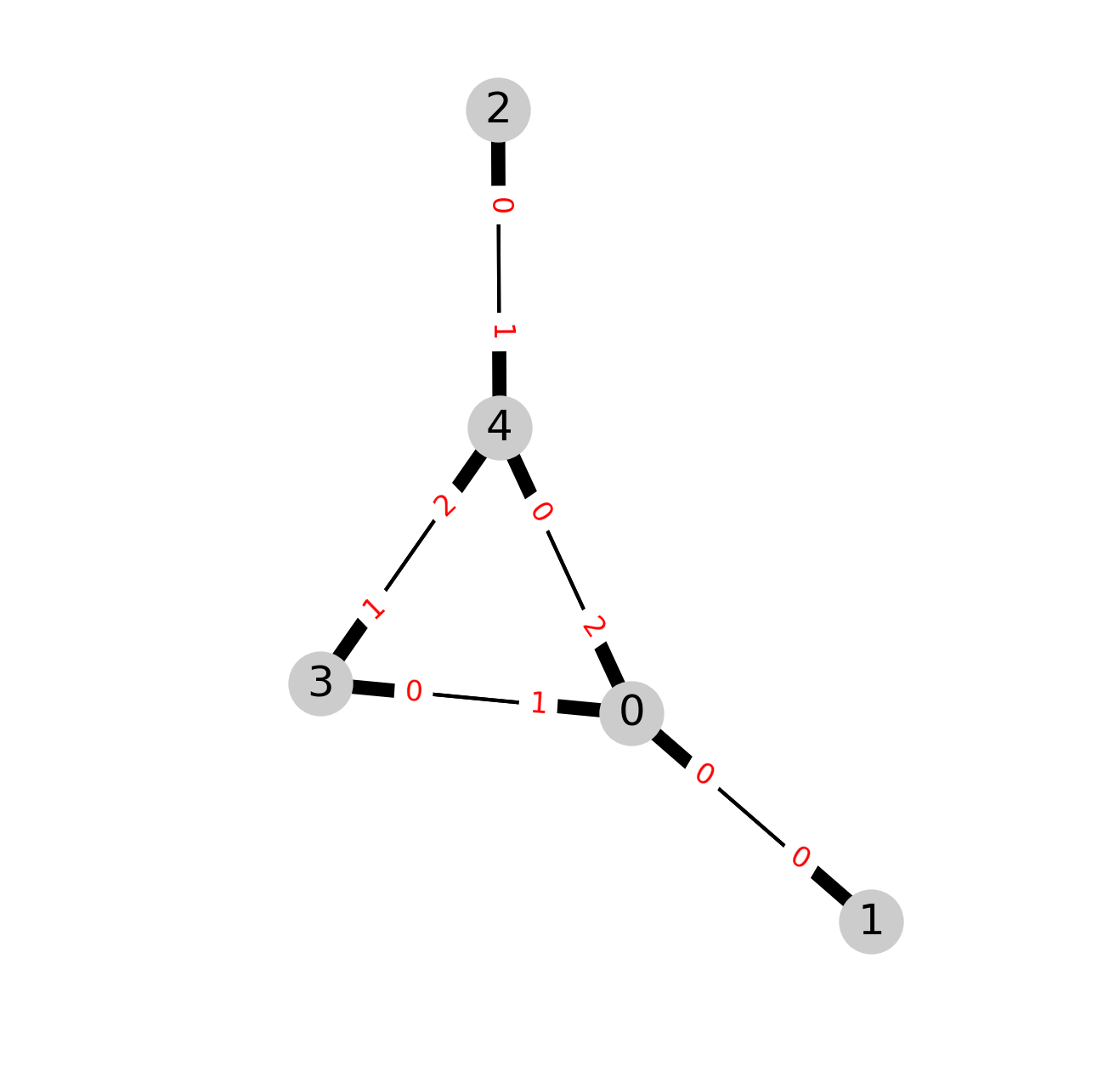
The figure shows a “bull” graph with the coding of nodes,

$$G = \{(1,3,4), (0), (4), (0,4), (0,2,3)\}\,,$$

and the corresponding connecting subnodes colors,

$$S = \{(0, 0, 0), (0), (1), (1, 2), (2, 0, 1)\}\,.$$

The distribution of degree is,

$$D = \{3,1,1,2,3\}\,.$$

Quantum state

The particle state is defined by two quantum numbers: position (vertex $x$) and internal state (coin state $c$).

$$|x,c\rangle \in \mathcal{H}_x \otimes \mathcal{H}_c$$

where $x=0,\ldots,N-1$ and $c=0,\ldots,d_x-1$.
We associate to each node of $G$ a spin state $|s_x\rangle$ that can take two values $s_x = \{0,1\}$. The spin state of the graph can be encoded by a binary string:

$$|s\rangle = |s_0\ldots s_x \ldots s_{2^N-1}\rangle$$
The basis vectors of the system’s quantum state is then defined by the kets,

$$|xcs\rangle$$

from which an arbitrary state can be written as a superposition of complex amplitudes $\psi_{xcs}$:

$$|\psi\rangle = \sum_{x,c,s} \psi_{xcs} |xcs\rangle$$

Remark

In order to define the hilbert space the coin number is extended at each node to $d_{M}$ values; operators will act as the identity over the (unphysical) extra degrees of freedom ($d_x,\ldots, d_{M}-1$), and the amplitudes corresponding to these base states, set equal to zero.

The coin and motion operator

Two interesting choices for the coin operator are the grover $\mathrm{GR}$ and fourier $\mathrm{FR}$ operators. The grover operator do not change the amplitudes of an equally weighted subnode state (it is not a balanced coin, but it is symmetric and respects the symmetries of the graph); the fourier operator equally distributes the amplitude at $x$ over the subnodes (it is a balanced coin, like the one used in the classical random walk).

For a node with $d_x$ incident edges, the elements of the grover matrix are defined by

$$\langle c |\mathrm{GR} | c' \rangle = \frac{2}{d_x} - \delta_{c,c'}$$

where $c,c'=0,\ldots,d_x-1$ are colors of node $x$.

The elements of the fourier matrix are,

$$\langle c |\mathrm{FT}| c' \rangle = \frac{1}{\sqrt{d_x}} \exp (\I 2 \pi c c' / d_x)\,.$$

The position operator (motion) swaps the state between two vertices $(x,y)$ of an edge according to the respective values of its subnodes $c(y)$ (pointing to the $y$ neighbor of $x$) and $c(x)$ (pointing to the $y$ neighbor $x$):

$$|xc(y)\rangle\; \rightarrow \;|yc(x)\rangle\,, \quad \forall y \in Y_x$$

where $Y_x$ is the set of neighboring vertices of vertex $x$.

The particle-spin and spin-spin interactions

We consider, at each vertex $x\in V$, a $1/2$-spin interacting with its neighbors $y \in Y_x \subset V$. The spin-spin interaction is of the magnetic exchange type, and is represented by the unitary operator controlled phase $\mathrm{CZ}$:

$$\mathrm{CZ} = \mathrm{diag}\,(1,1,1,-1)$$

that acts on pairs of qubits, taking the first one as control; it changes $|11\rangle\;\rightarrow\;-|11\rangle$, letting the others pairs unchanged.

In general the spin state local to a vertex is a superposition of base states:

$$|s\rangle = |s_0 s_1\ldots s_{N-1}\rangle,\quad s = s_0 + s_1 2 + s_2 2^2 + \cdots + s_{N-1} 2^{N-1}$$

The spin-particle interaction is given by a swap gate:

$$\mathrm{SWAP} = \begin{pmatrix} 1 & 0 & 0 & 0 \\ 0 & 0 & 1 & 0 \\ 0 & 1 & 0 & 0 \\ 0 & 0 & 0 & 1 \end{pmatrix}$$

extended to the appropriated dimension, depending on the node degree $d_x$. Its action on the base state is to exchange the first coin qubit $c=0,1$, with the local spin $s_x=0,1$, qubit,

$$|x,c=1,s_0 s_1 \ldots s_x=0 \ldots s_{N-1}\rangle \; \rightarrow\; |x,0,s_0s_1\ldots 1 \ldots s_{N-1}\rangle$$

and similarly with $c = 0 \rightarrow s_x=1$.

Summary

Therefore, the hilbert space is spaned by base states of the form,

$$|xcs\rangle\,,$$

with

a node (position) number $x = 0,\ldots, N-1$;
a coin number $c = 0, \ldots, d_x-1$ (extended to $d_M=\max{d_x}$);
and a the set of binary digits $s=0,\ldots, 2^N-1$, defined on a graph $G=(V,E)$

The evolution of the quantum state is ruled by (schematically) the following operations:

a mixing of the color state $|xcs\rangle\rightarrow \sum_c |xcs\rangle$;
an interchange of the states of two adjacent nodes, $|xc(y)s\rangle \rightarrow |yc(x)s\rangle$;
a swap of color and spin at each node, $|xcs_x\rangle \rightarrow |xs_xc\rangle$;
and a phase $-1$ for two neighboring down spins, $|xc1\ldots 1 \rangle \rightarrow -|xc1 \ldots 1\rangle$.

Evolution of the quantum state

Graphs

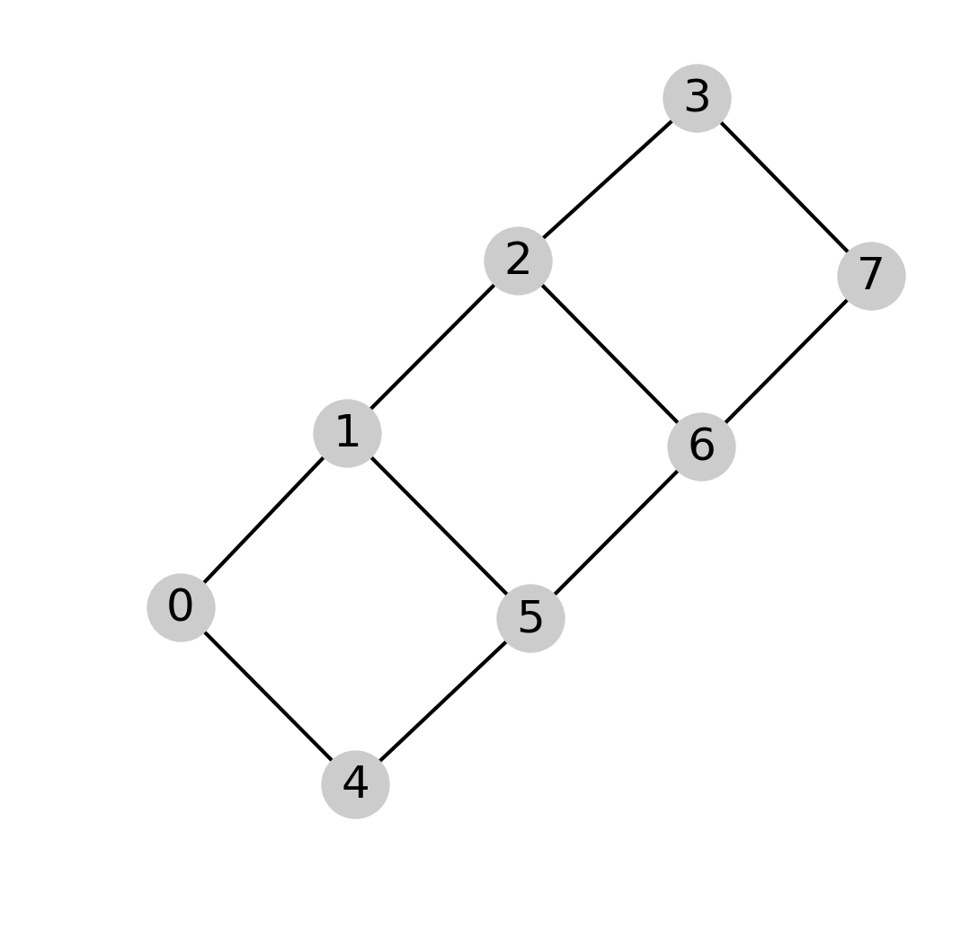
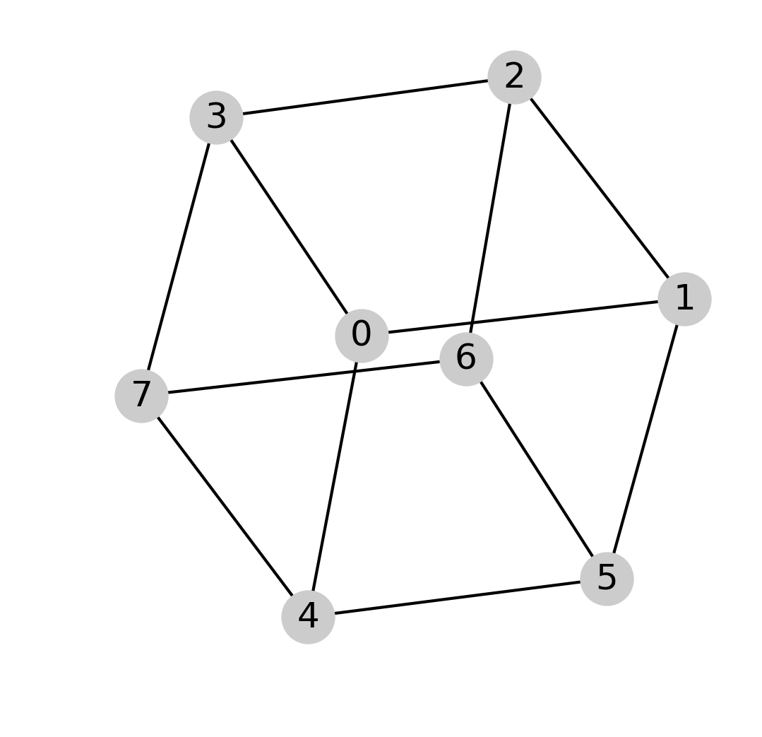
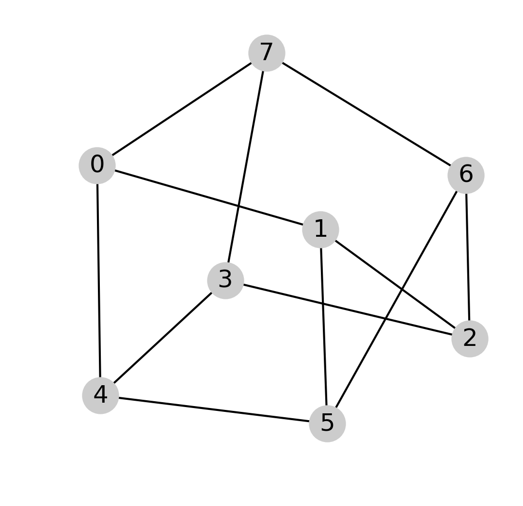
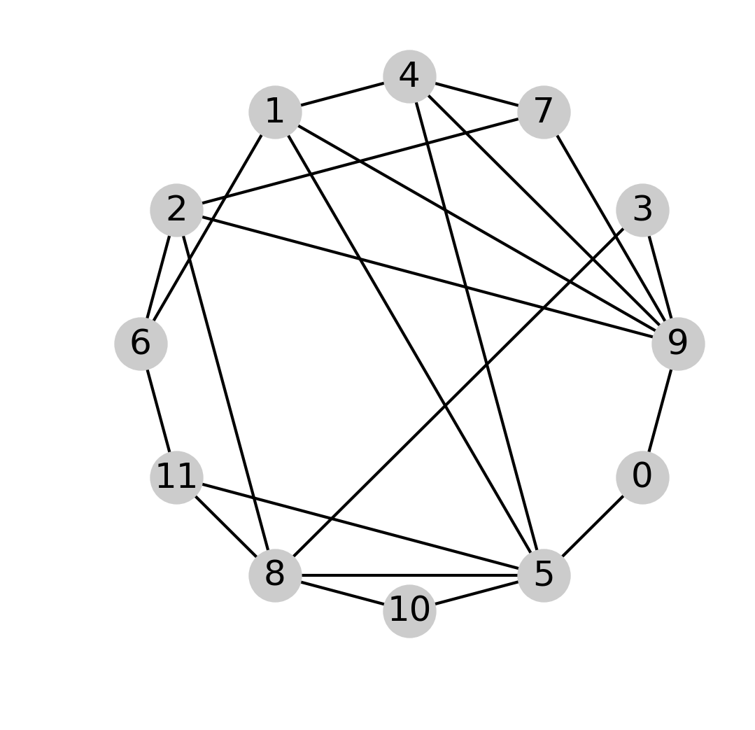
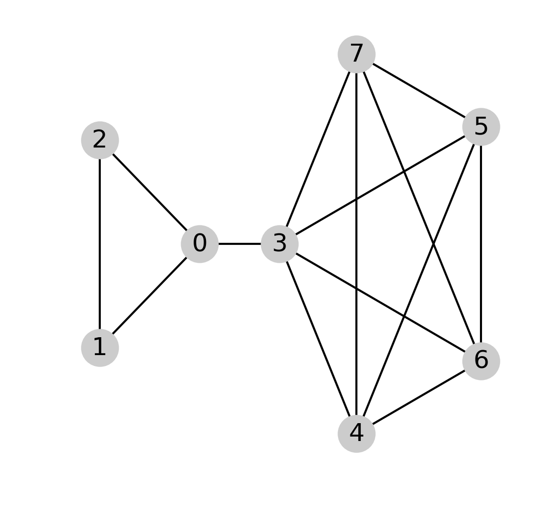
Some typical graphs:


“ladder”	“cube”	“moebius”

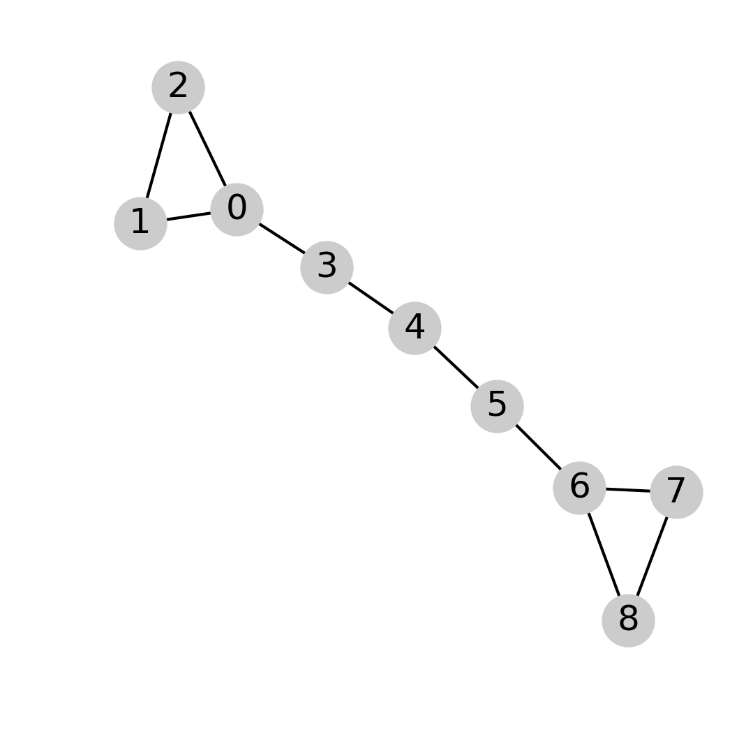“random”	“kite”	“chain”

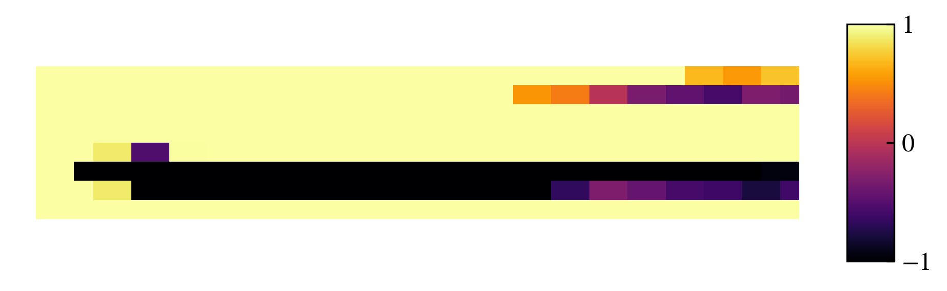
Position and spin distributions

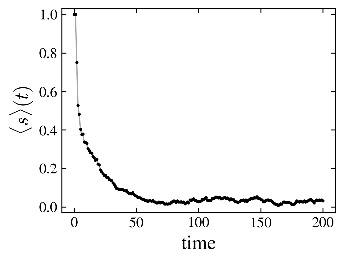
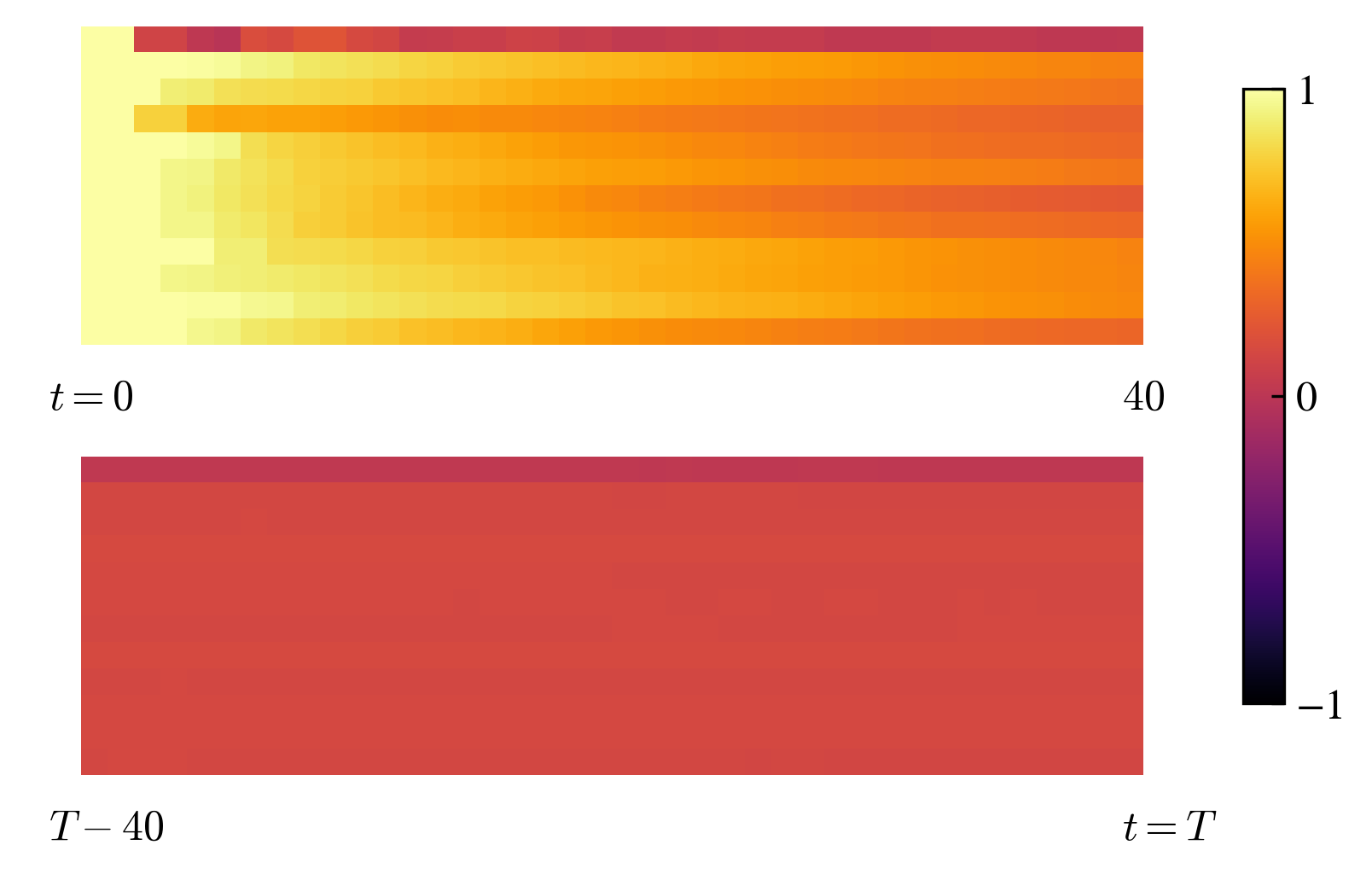
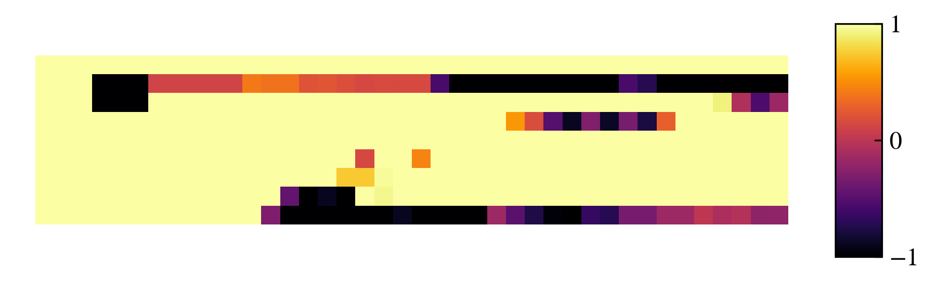
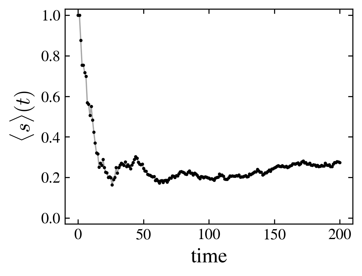
The initial state is $|000\rangle$. After a transient, the state evolves towards a stationary state with a definite mean spin and a stable probability distribution over the nodes (which may be a cycle)


“ladder”

“random”

“chain”
First steps of the spin distribution over the nodes (horizontal axis is time, vertical axis is node)	Mean spin

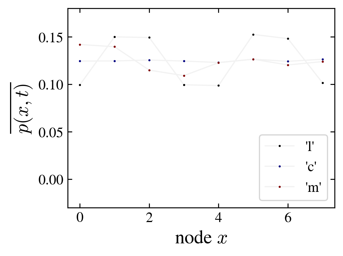
The position probability at node $x$ and step $t$ is,

$$p(x,t) = \sum_{cs} |\psi_{xcs}(t)|^2\,,$$

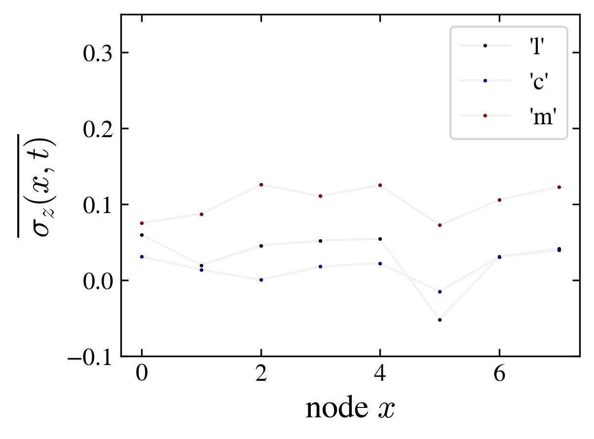
the spin distribution,

$$s(x,t) = \langle\sigma_z\rangle (x,t) = \sum_{yc} \big(\sum_{ \{s,s_x=0\} } |\psi_{ycs}(t)|^2- \sum_{ \{s,s_x=1\} } |\psi_{ycs}(t)|^2 \big) \,,$$

Using the density matrix $\rho = |\psi(t)\rangle \langle \psi(t)|$, we may write the above equations in a compact form,

$$p(x,t) = \mathrm{Tr}_{cs}\, \rho\,,\quad s(x,t) = \mathrm{Tr}_{xc} \, \rho \sigma_z$$

where $\mathrm{Tr}_x$ is the partial trace over the $x$ hilbert space.

Exact spectrum of $U$

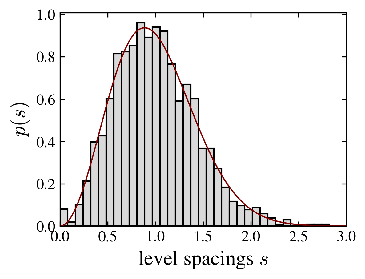
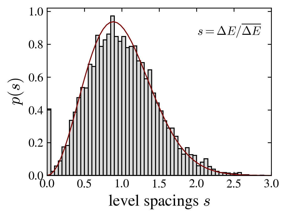
The spectral properties of the evolution operator correspond to random matrix ensembles. For most graphs, the level spacing distribution is well fitted by the Wigner surmise of the gaussian unitary ensemble.


“ladder”	“random”	“chain”

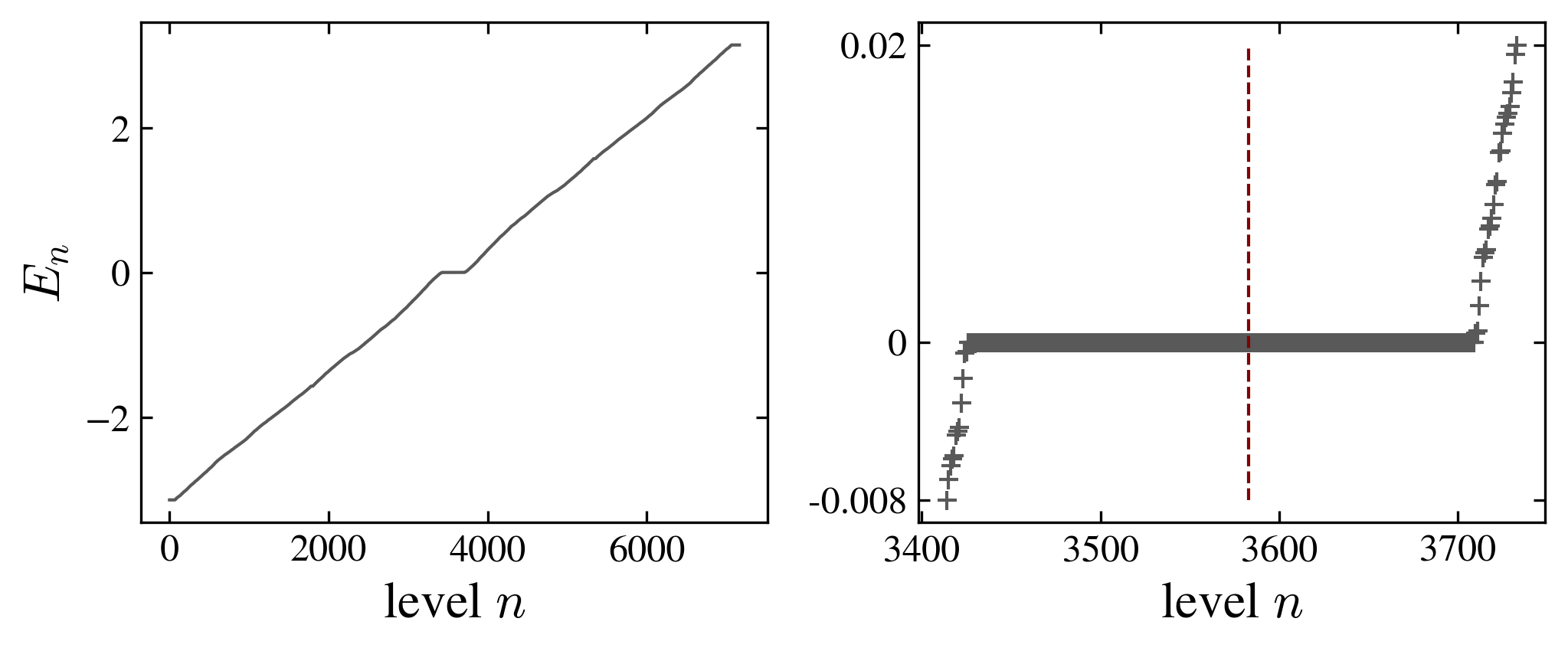
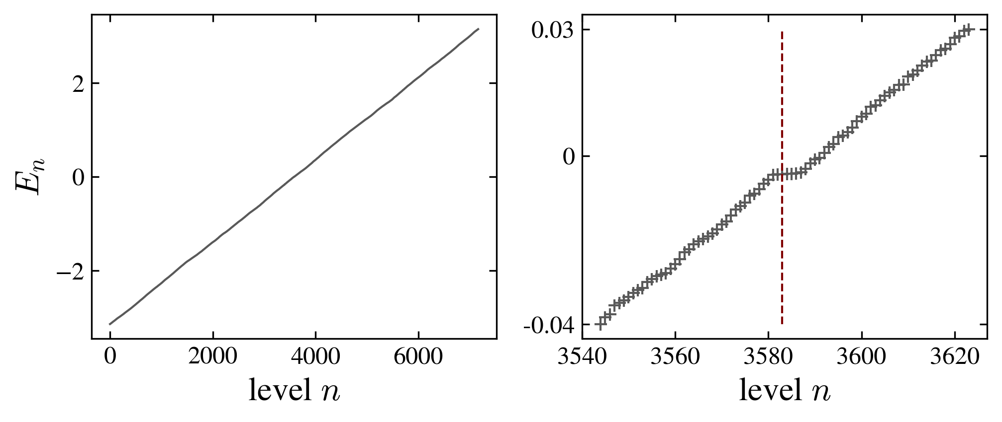
We compute numerically the exact spectrum of the operator $U$:

$$U|n\rangle = \E^{-\I E_n} |n\rangle$$

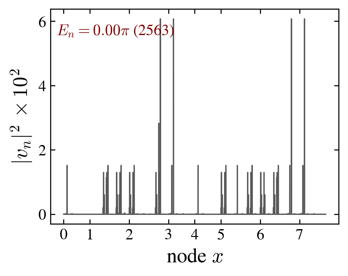
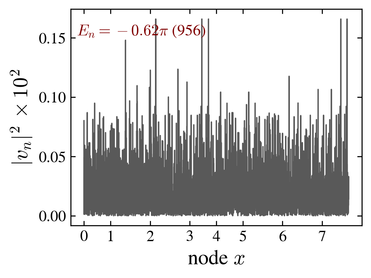
where $E_n$ is the quasi-energy $E_n\in[-\pi,\pi]$, and $|n\rangle$ the corresponding eigenstate. We denote $v_n$ the complex eigenvector of level $n$ in the $|xcs\rangle$ representation:

$$v_n(xcs) = \langle xcs | n \rangle$$

which are the columns of the change of base matrix (from $|xcs\rangle$ to $|n\rangle$).

The spectrum $E_n$ may contain a mixture of degenerate eigenvalues (in particular at $E_n=-\pi,-\pi/2,0,\pi/2,\pi$) and randomly spaced eigenvalues filling the circle; eigenvectors corresponding to degenerate eigenvalues are localized while a typical eigenvector is “thermal”.
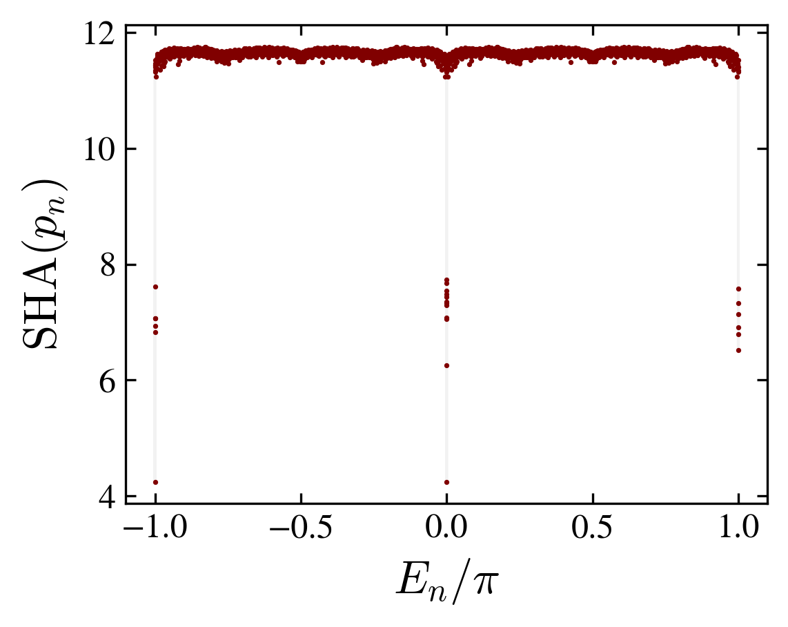
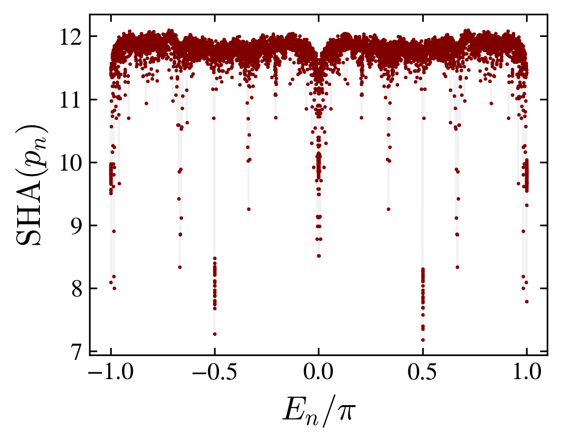
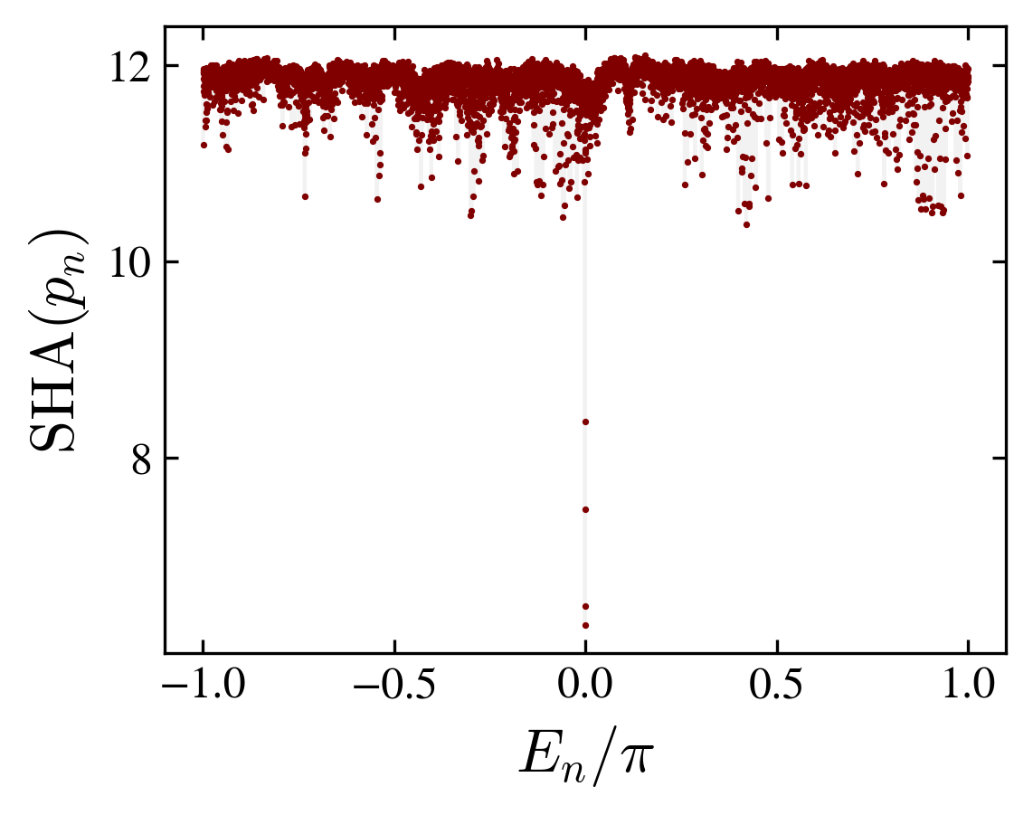
From the eigenvectors of $U$, we can define a Shannon entropy using $p_n=|v_n|^2$ as the probability distribution. The Shannon entropy $\mathrm{SHA}$, is a measure of the typicality:

$$\mathrm{SHA}(n) = - \sum_{xcs} |v_n(xcs)|^2 \log|v_n(xcs)|^2$$

We adopt as a definition of “thermal eigenvectors” such corresponding to a maximum Shannon entropy.


“ladder” $E_n = 0$ eigenvector	“ladder” maximum Shannon entropy eigenvector

Thermalization

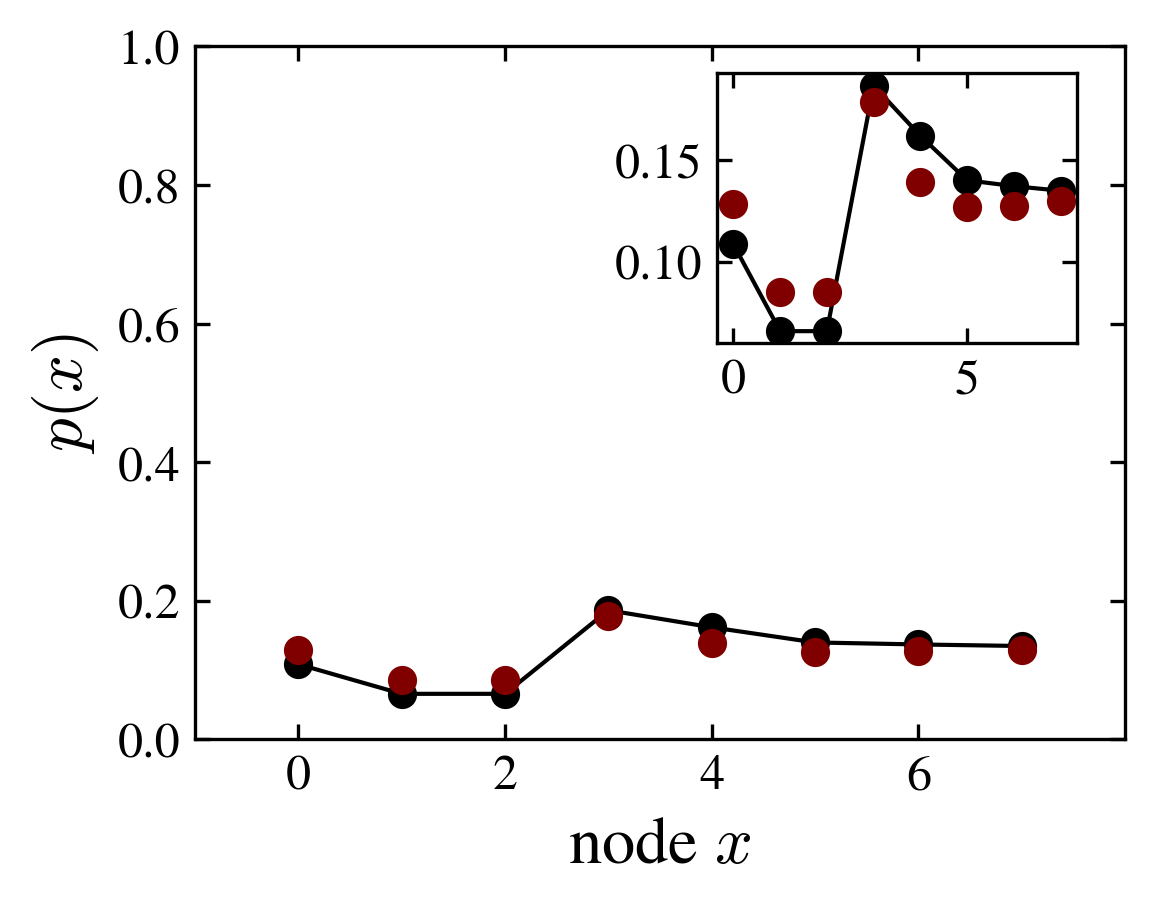
Thermal eigenvector hypothesis. It was originally formulated by Srednicki and Deutsch. According to this hypothesis the relaxed (long time) value of an observable $M$ coincides with its expectation value in one typical energy eigenstate:

$$\langle \psi(t)|M|\psi(t)\rangle \approx \langle n|M|n\rangle\,.$$

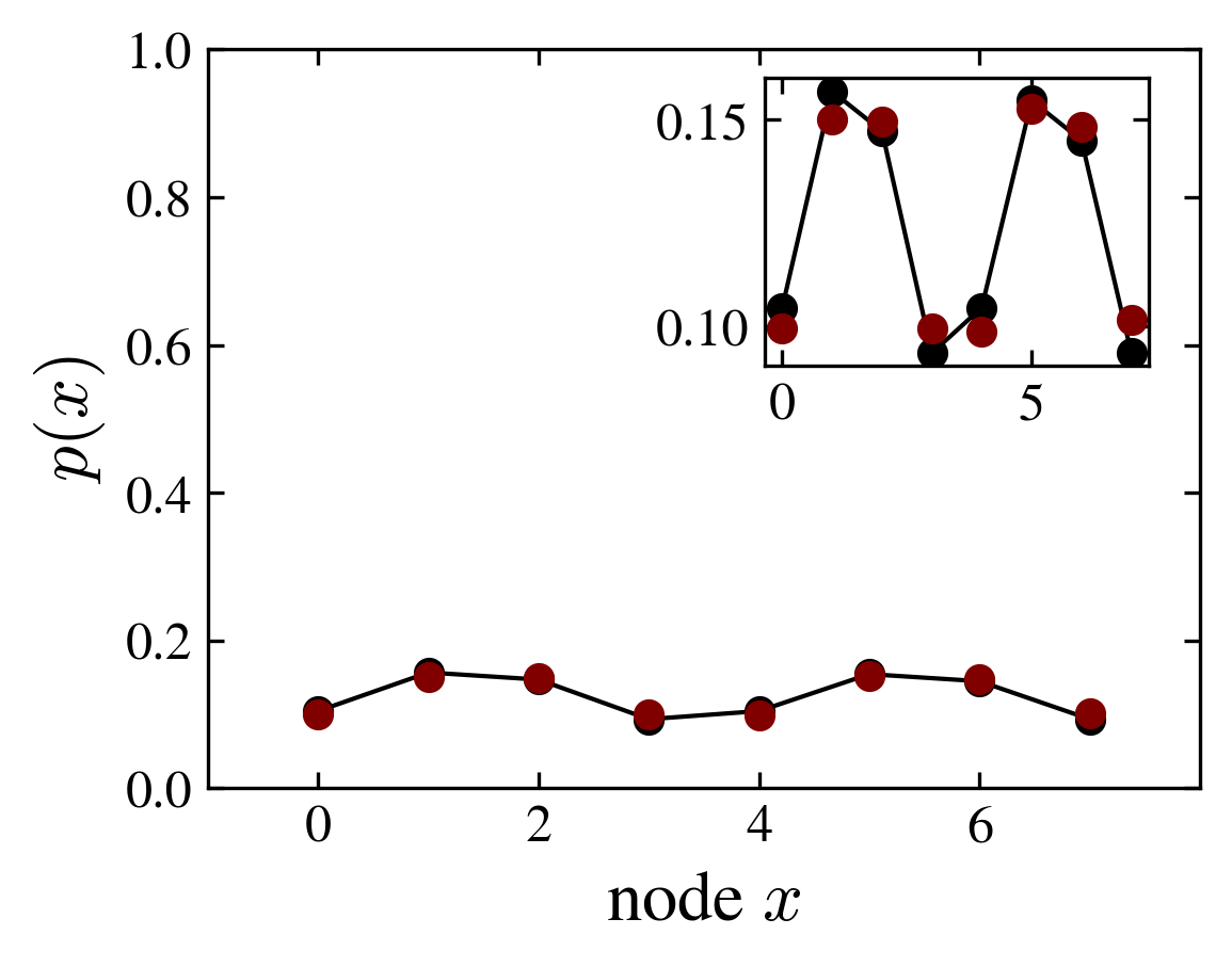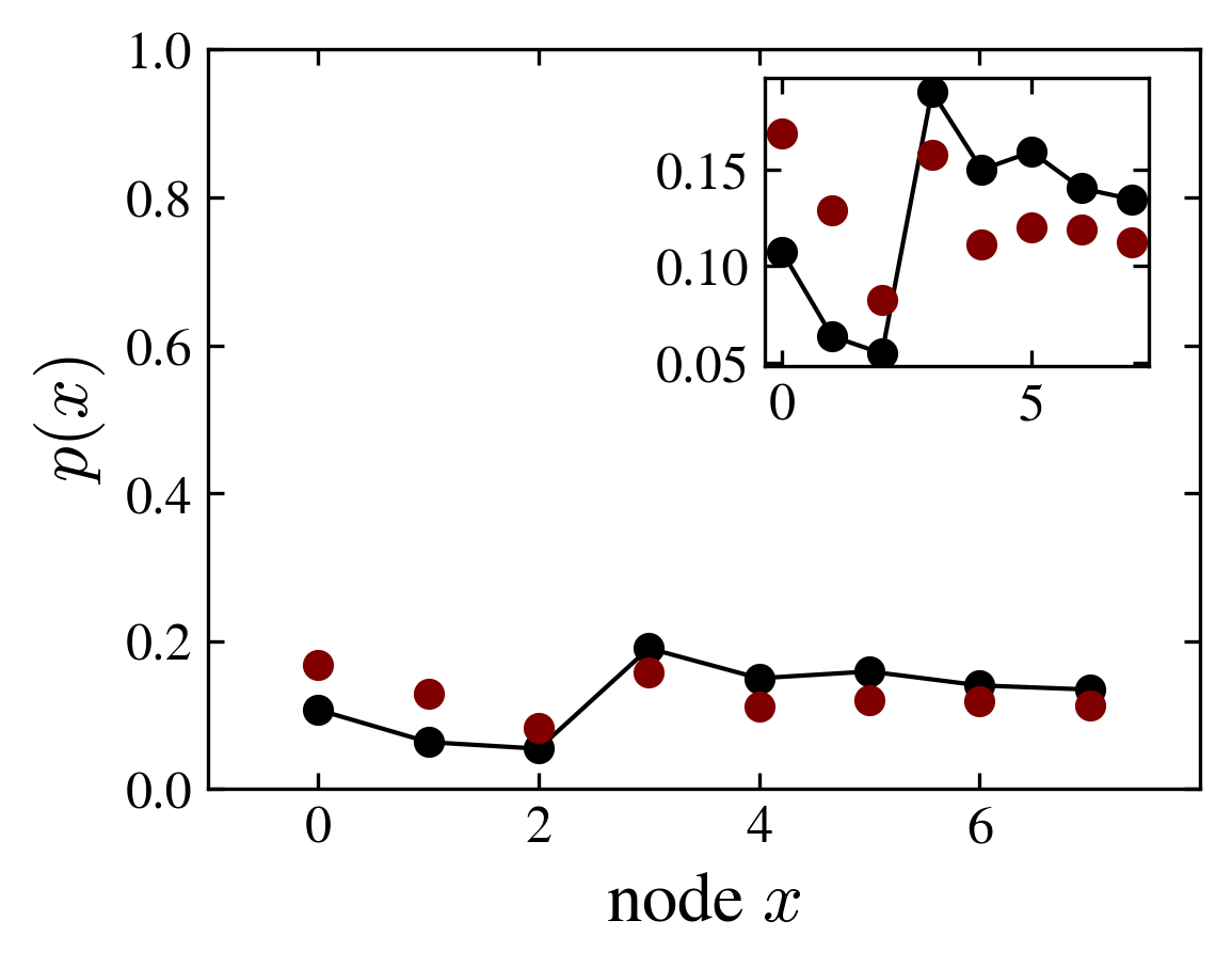
The figure shows the position probability distribution of the ladder graph, numerically computed using the evolution operator and averaged over time (red points); and computed using only one eigenvector (solid line, black points). The selected eigenvector is the one having maximum Shannon entropy.

Remark

One usual requirement of (thermal) equilibrium is homogeneity. In the present model “homogeneity” must be understood as uniformity compatible with the graph connectivity. In the case of the grover coin, the equilibrium distribution of the position probability depends on the degree distribution:
$$p(x) = d_x/\sum_x d_x$$

The cube and moebius graphs

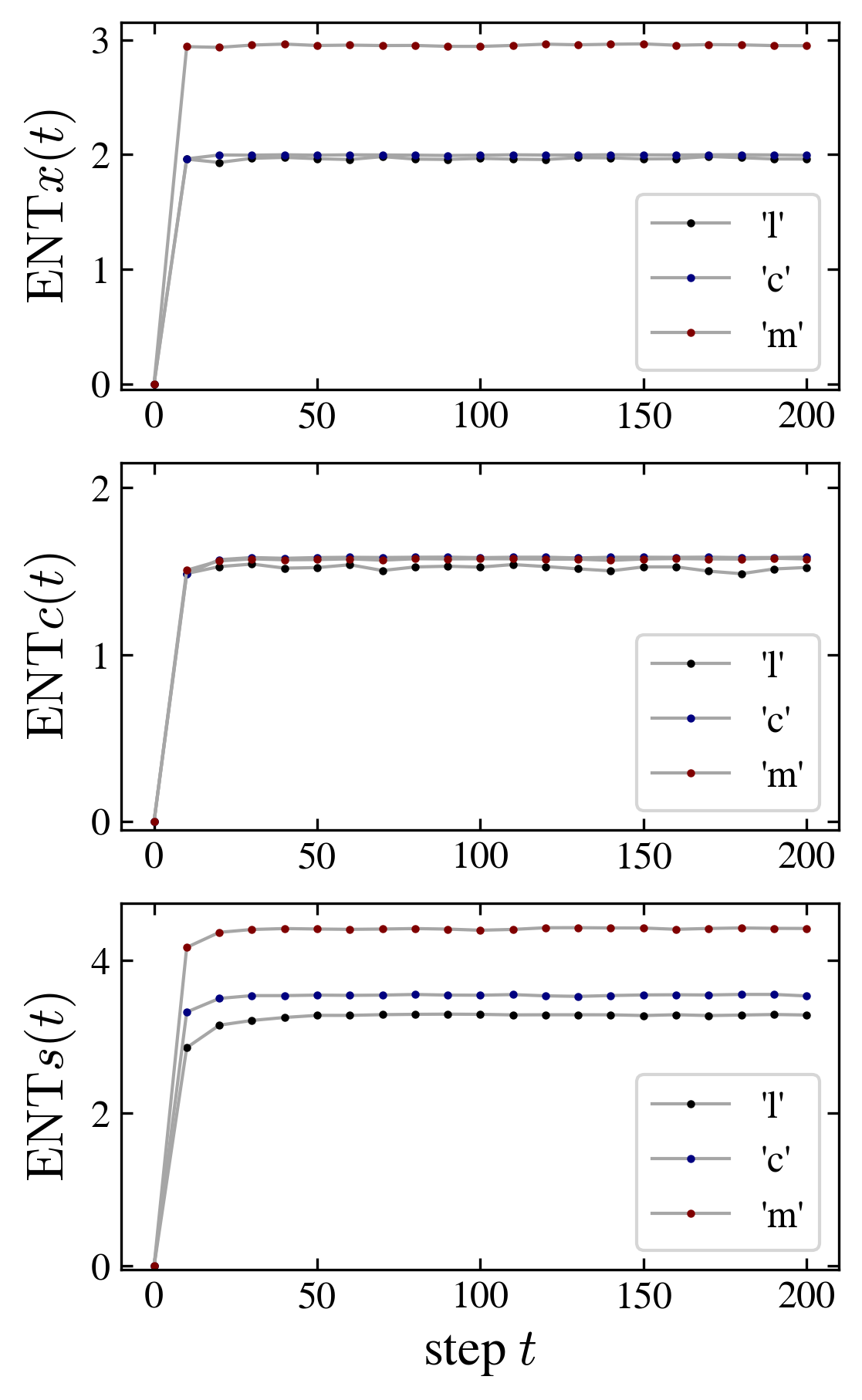
The entanglement and thermalization properties depend on the topology of the graph. A comparison of the “cube” and “moebius” graphs illustrate this effect.

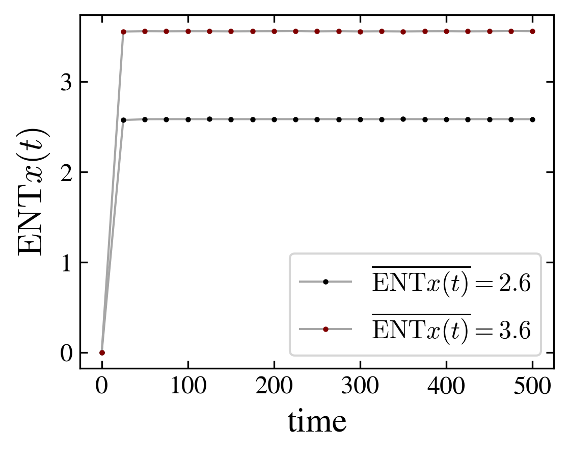
To characterize the entanglement between the walker and the graph spins, we measure the von Neumann entropy

$$\mathrm{ENT}x(t) = - \mathrm{Tr}\, \rho(x,t) \log \rho(x,t)\,,\quad \rho(x,t) = \mathrm{Tr}_{cs}\,\rho(t)$$

for the particle entanglement entropy, and similar formulas for $\mathrm{ENT}c$ (coin entropy) and $\mathrm{ENT}s$ (spin entropy).

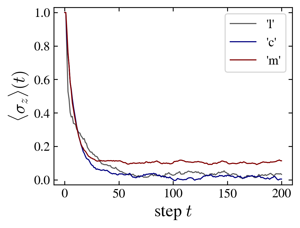
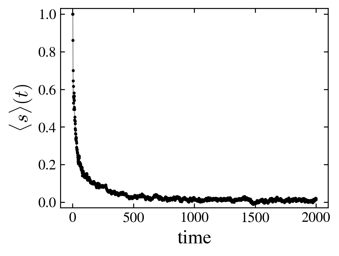
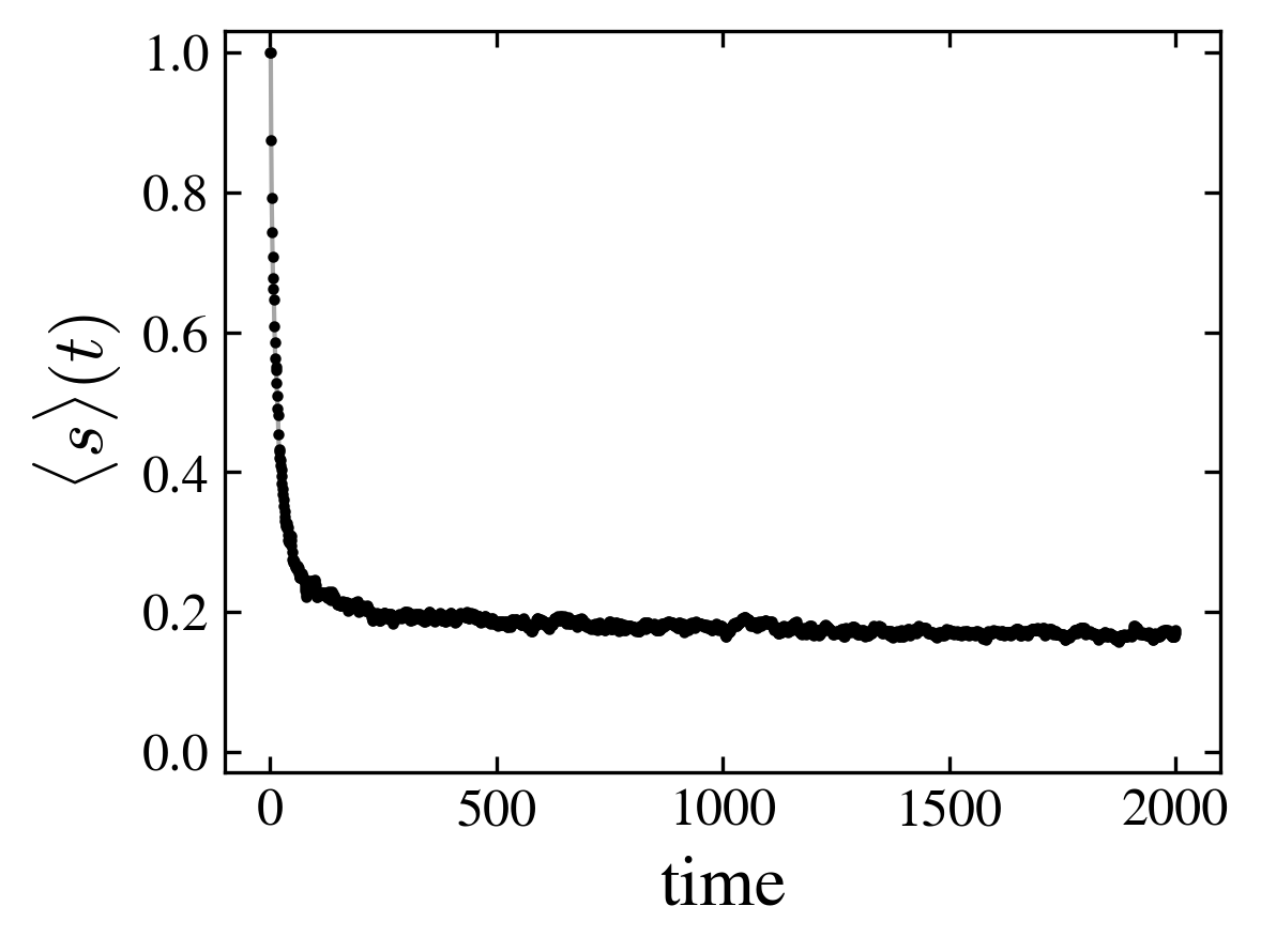
The cube (as well as the ladder graph) tends to a paramagnetic state (mean zero spin, uniform distribution) while the moebius tends to a ferromagnetic state (finite positive magnetization, uniform distribution over the nodes). These differences in the magnetic properties go together with a difference in the entanglement (figure).




Entropy of the “position”, “color” and “spin” subsystems (left); mean position and spin probabilities over the nodes, and averaged spin (right), for the ladder, cube and moebius graphs.

Adopting for the moment a classical statistical mechanics reasoning, one notes that the relaxation of the initial state (particle at node $x=0$, and uniform spin up distribution over the graph, $s=0$) follows the behavior of a system governed by ferromagnetic interactions, no staggered magnetization is observed. In addition, the system behaves as if there were an effective finite temperature depending on the graph’s topology. Actually, both graphs have the same degree distribution and connectivity, but the cube is a plane graph, but not the moebius which possesses one crossing. However, this “explanation” is not well justified for the present model. Indeed, the model being defined by a unitary operator split into elementary transformations acting on the quantum state, the existence of a (local) hamiltonian from which a standard thermodynamic argument might be build, is not guaranteed. One may, instead, think the apparent thermodynamic behavior as emerging form the system’s “dynamics”.



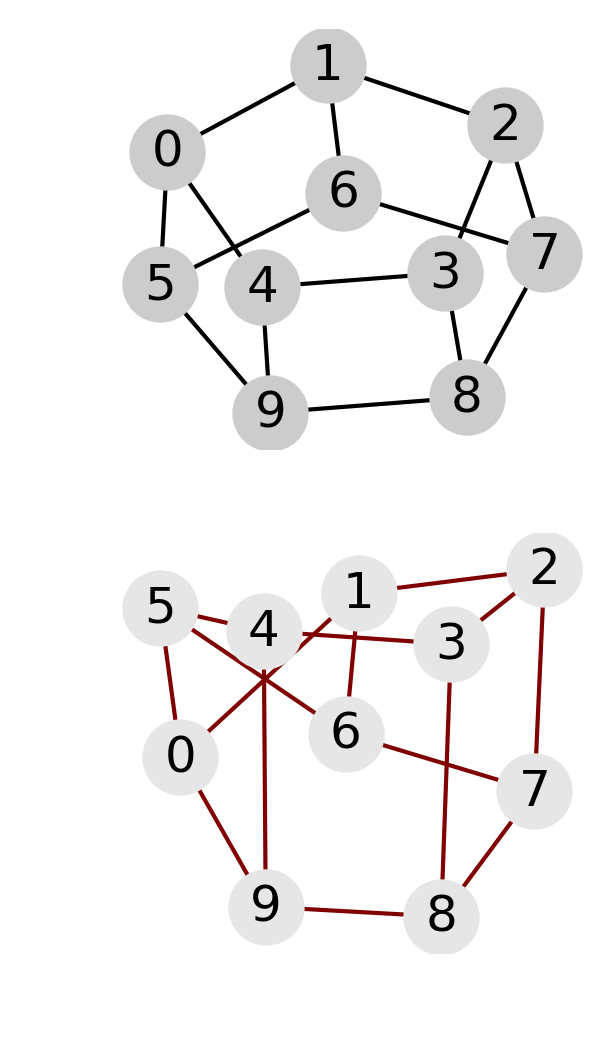
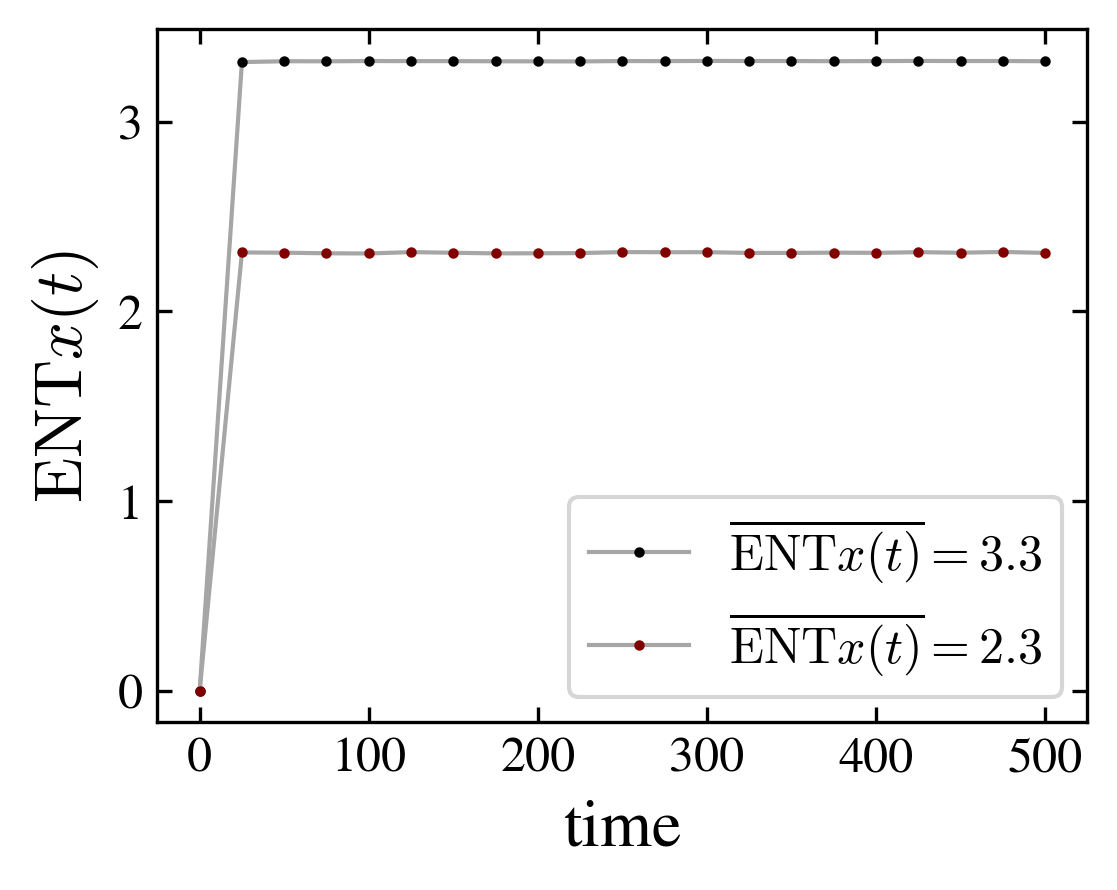
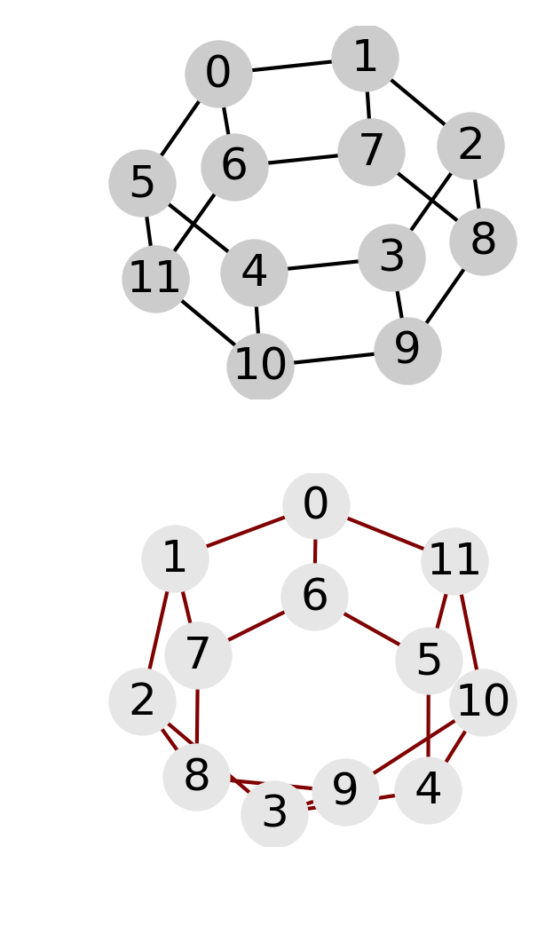
Periodic and crossed ladder graphs with 10 and 12 nodes. For the 10 node graph an increase of magnetization for the crossed graph is correlated with a decrease of the position entanglement entropy. The opposite effect is observed for the 12 node graph: in this case, periodic and crossed graphs behave similarly to the cube and moebius graphs, respectively

In fact the relation interaction-entanglement is more complex. Considering the same type of graphs, a ladder with periodic (i.e. cube) or crossed (i.e. moebius) boundary edges, but with increasing number of nodes, one observes two distinct effects of the interaction: it can be related to entangled magnetic order, or to unentangled magnetic order. Indeed, depending on the number of nodes, entanglement entropy and magnetization are correlated or anticorrelated, as shown in the above figure. However, in both cases the magnetization is the same for the respective, periodic or crossed, graphs, and the change in the entanglement entropy is of the same magnitude, $\Delta \mathrm{ENT} = \pm 1$; the plus sign applies to the 8 and 12 graphs and the minus sign to the 10 nodes graph.

The kite graph

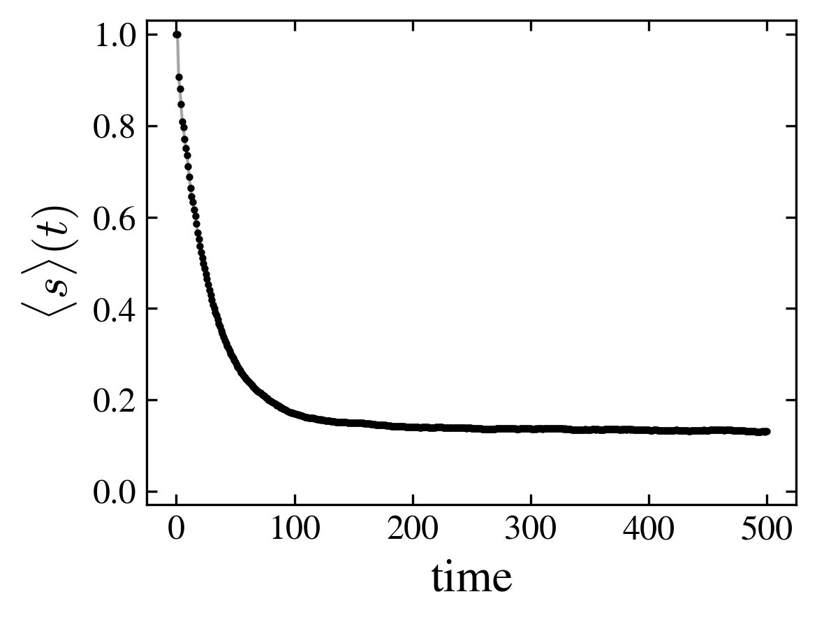
The magnetic relaxation depend not only on the graph topology (as in the case of the cube and moebius) but on the coin operator. For the “kite” graph the relaxation towards the paramagnetic state is much slower for the fourier coin than for the grover one, even if in the two cases the state tends to be paramagnetic at long times.


Grover coin	Fourier coin

At variance to the cube-moebius case for which the entanglement entropy differs between the two magnetic states, in the present case, the entropy remains of the same order for the two coins, in agreement with the observation that the asymptotic state is paramagnetic.

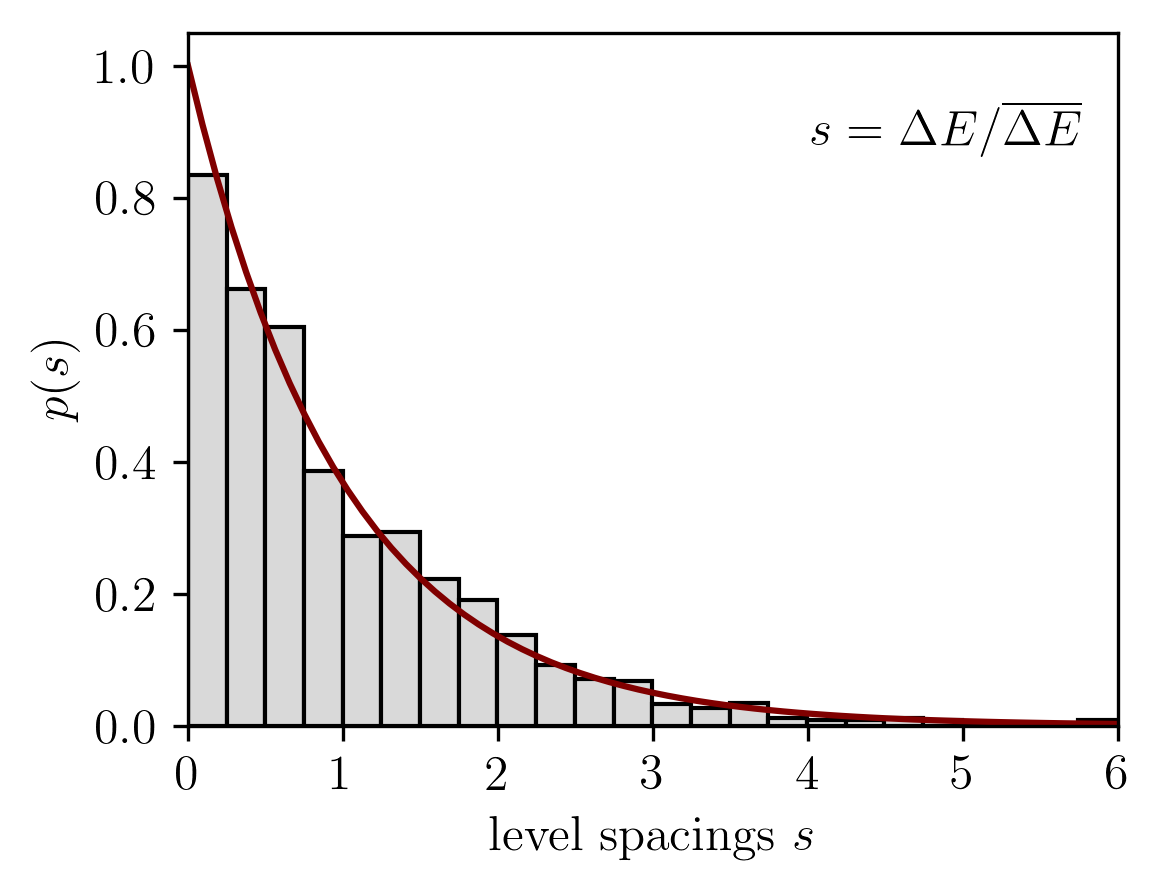
The coin also has an influence on the degeneracy of levels; in particular the fourier coin breaks the geometric symmetries of the graph, suppressing almost completely the degeneracy of the spectrum.

Grover coin (top) and fourier coin (bottom)

Shannon entropy and probability distribution compared with one eigenstate estimation (thermal hypothesis)



Grover coin	Fourier coin

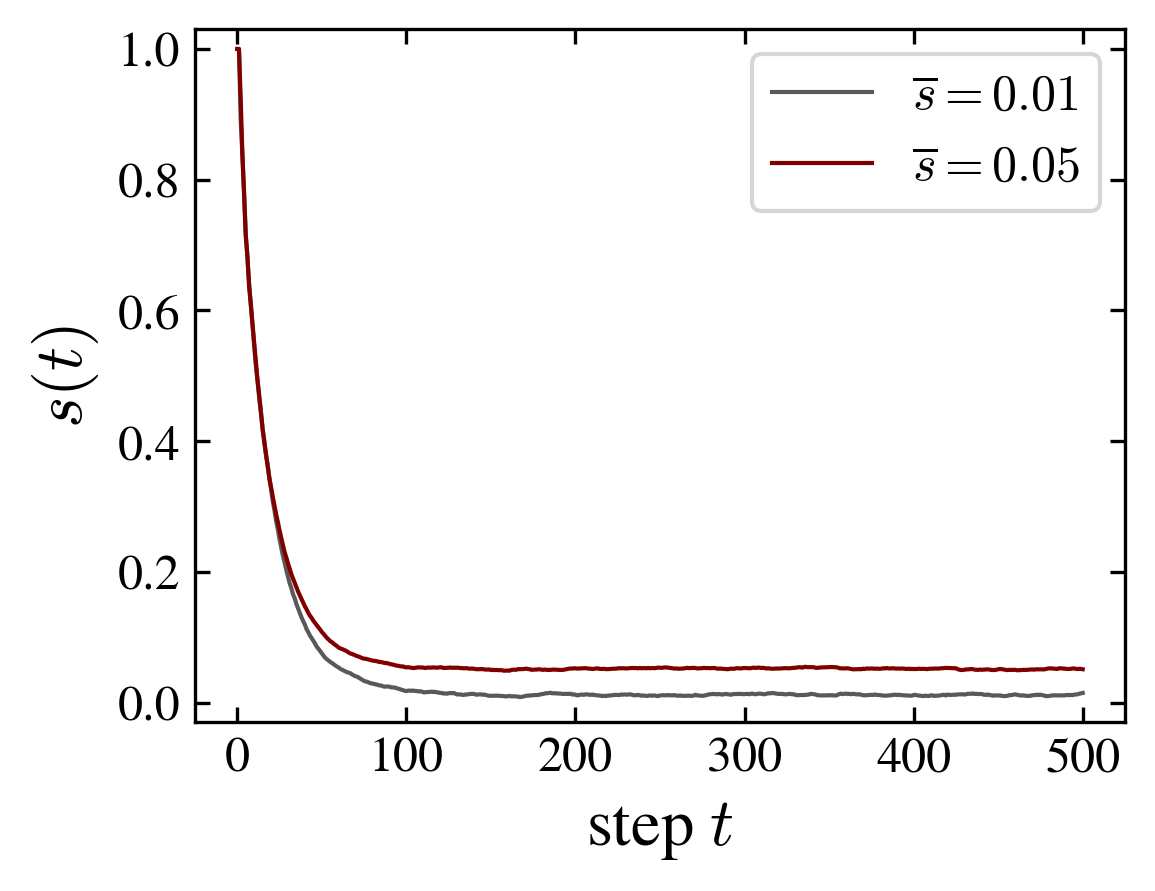
Although the kite graph with a fourier coin slowly relax, it approaches at finite times, a thermal state with small fluctuations related to a (decaying) overlap with the initial state.

One condition for thermalization is the random nature of energy (here quasi-energies) eigenvectors: the effective hamiltonian behaves as a random matrix. We verified that the phase distribution of the complex vectors is effectively random, and uniformly distributed on the circle.

Discussion

The origin of the thermalization (we call it thermalization, even if the reached stationary state is not the Gibbs one) is the interplay between the local rules governing the interaction and change of the quantum state, and the nonlocal entanglement these same rules create. The rules are strictly local: motion by swaps between neighbors, spin-spin and spin-particle exchange, however the quantum dynamics, the action of the unitary $U$ operator, is global, it applies on the full hilbert space. The grow of the quantum state complexity is measured by the entanglement entropy, larger the entanglement, more complex stationary states are possible. For instance, the difference of one qubit between the thermal state of the cube and the asymptotic state of the moebius, translates in a trivial paramagnetic state for the cube and a ferromagnetic state (with finite effective temperature) for the moebius. The shuffle of the amplitudes ensured by the (parallel) unitary step operator, associated with the specific geometric properties of the graph, create an entangled state whose complexity increases without the need of external perturbations or quenched randomness, or even averaging over initial conditions.

Measures are local, but depend through the actual quantum state on the whole effective hilbert space (and on the whole history of the interactions). The system statistically projects under successive application of $U$, into one of the typical eigenvectors of $U$, which are by definition invariant under the evolution. As a consequence, a measure that is also by definition local, results in an averaging (partial trace) over a complex (thermal) whole hilbert space eigenvector. Accessibility of local information of a nonlocal entangled state (partial information of a global correlated system) is at the heart of the effective thermal behavior of observables.

It worth noting that the usual definition of thermalization in isolated quantum systems is based on the microcanonical ensemble, and therefore it is tightly related to the system’s energy: the thermal state is a hamiltonian eigenstate corresponding to the neighborhood of the mean energy eigenvalue. In our model there is no local hamiltonian, and no obvious energy related to the initial configuration. However, the natural definition of a thermal state in terms of the entropy maximization, revealed to be sufficient to identify the thermal state.


“ladder”	“cube”	“moebius”

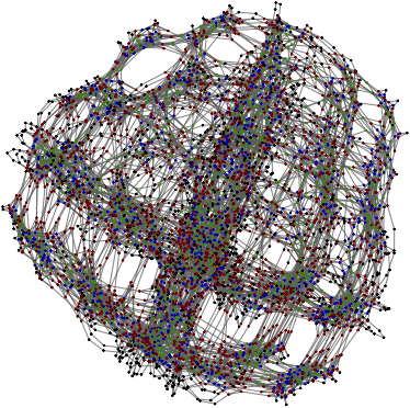
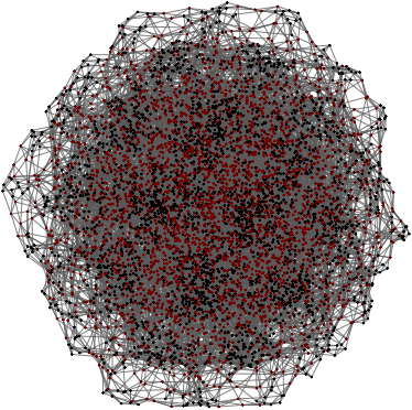
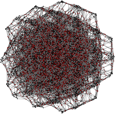
To explore the structure of the hilbert space we associate to the step operator $U$ a graph $G(U)$; the elements of the matrix representing $U$ are associated with the nodes of $G(U)$. The question is whether the statistical properties of $G(U)$ are related to the thermalization properties of $U$.


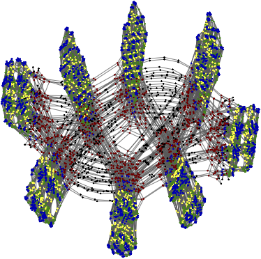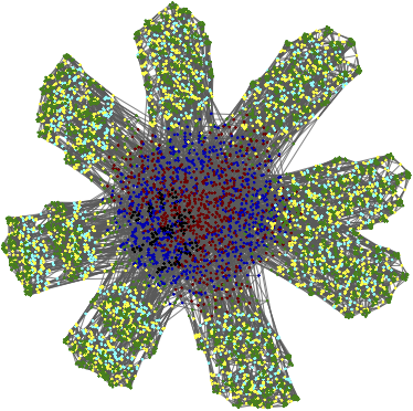Kite graph (grover), nodes are colored by degree $d=\{2,4,7,8,9\}$	(fourier), $d=\{3,4,5,7,8,9\}$ (black, red, bleu, green, yellow, cyan)

The role of interactions in establishing a “generic” or “typical” state is double. Interaction can, on one side, generate entanglement, leading to correlated ordered macroscopic states (uniform density and finite magnetization), but, on the other side, interaction can destroy entanglement and favor an ordered state (with finite magnetization) which is closer to a product state. Order is no synonym of entanglement, nor it is synonym of interaction (as in the mean field description of thermodynamic phases).

Conclusion

A traditional approach to quantum systems is to start from a classical point of view (Bohr); within this framework, supported by the correspondence principle, a classical hamiltonian is transformed into a quantum one by replacing the Poisson bracket between canonical variables by the corresponding commutator between operators (Dirac). However, the reasoning consisting in comparing classical and quantum systems obviously has its limitations. For instance, after the discovery of chaos in simple dynamical systems, it appeared as natural to ask whether the associated quantum systems also showed chaotic behavior (Berry, 1987). Soon it was apparent that new phenomena arised in quantum systems without equivalent with classical mechanisms (dynamical localization in the kicked rotator, for example, Casati and Izrailev).

Our starting point in this work reverses this traditional approach: we define, using the elementary principles of quantum mechanics, a system satisfying a set of simple unitary transformation rules, and ask whether it can exhibit some ordered collective behavior. We observed that the interplay of interaction and entanglement, respectively local and nonlocal mechanisms, lead the system to a variety of states that can be characterized by well defined measurable properties: spatial distribution of the probability, magnetic order, thermalization.

It is yet an open question to explain by which specific mechanisms the topology of the hilbert space graph does influence these properties.

Notes

Chaos: in a very schematic way, valid in the semiclassical approximation, one may say that the signature of integrability is a Poisson distribution of the level spacings; and that quantum chaos is instead characterized by the Wigner-Dyson ensembles (see for instance Haake, Qunatum signature of chaos). Beyond this operational definition, quantum chaos can be related to the cause a quantum system behaves statistically as stated by van Kampen. Definitions based on the semiclassical limit are not relevant: the long time and high quantum numbers (or formally $\hbar \rightarrow 0$) limits do not commute; moreover

The process of quantizing a classical Hamilton system is not unique and does not correspond to anything in nature, which is fundamentally quantum mechanical (van Kampen, 1985).

We retain as a definition of quantum chaos the statistical behavior of the eigenvalues and eigenvectors (amenable to a description in terms of random matrices) of the system’s hamiltonian, and extend it to the unitary evolution operator (for systems where the hamiltonian is unknown or do not exists as a local operator, Dyson, 1962).

It is worth noting that integrability and statistical behavior are not related in quantum systems as in classical ones: observables may converge to their statistical (microcanonical) expectation value even for integrable systems. Indeed, the mechanism by which the system approach equilibrium is phase mixing, and it can take place for generic initial states in integrable systems, which negligible overlap with any of the hamiltonian eigenfunctions (Jansen & Shenkar, 1985]).
Ergodicity: for a closed classical system the time average of the trajectory $X(t)$ in phase-space (having energy $E$) is equivalent to the microcanonical expectation value of the density $\rho$,

$$\overline{\delta(x - X(t,E))} = \rho_E\,.$$

The straightforward generalization to quantum isolated systems,

$$\overline{|\psi(t)\rangle \langle \psi(t)|} = \sum_{n \in I(E)} |\psi_n|^2 |n\rangle \langle n| = \rho_\mathrm{diag} \,\overset{?}{=}\, \rho_E, \quad |\psi(0)\rangle = \sum_{n \in I(E)} \psi_n |n\rangle$$

is almost never realized, where we defined the so called “diagonal ensemble” $\rho_\mathrm{diag}$, which is in general distinct to the microcanonical one, $I(E)$ is a “small” interval around $E$, and $|n\rangle$ the energy eigenvectors. Von Neumann introduced the concept of quantum ergodicity at the level of observables:

$$\overline{\langle \psi(t)|M|\psi(t)\rangle } = \sum_{n \in I(E)} |\psi_n|^2 \langle n| M |n \rangle = \mathrm{Tr}\,\rho_\mathrm{diag}M = \mathrm{Tr}\,\rho_E M$$

where $M$ is a macroscopic (coarse-grained) observable (Polkovnikov et al. 2011).
Eigenstate thermalization hypothesis: for a chaotic isolated quantum system with energy $E$, the microcanonical expectation of a macroscopic observable, coincides with the expectation obtained from a single energy eigenstate:

$$\langle M \rangle = \mathrm{Tr}\, \rho_E M = \langle n|M|n\rangle$$

which means that the diagonal terms (in the energy base) of the observable $M$ are slowly and weakly varying, and that the off diagonal elements vanish in the thermodynamic limit. The thermal eigenstate hypothesis can be seen as a condition to the more stringent quantum ergodicity (Rigol and Srednicki, 2012). This hypothesis was numerically (Rigol, 2008) and experimentally (Kaufman, 2016) verified.

Random physics

Simple model of a complex quantum system

Remark

Quantum graph

Quantum state

Remark

The coin and motion operator

The particle-spin and spin-spin interactions

Summary

Evolution of the quantum state

Graphs

Position and spin distributions

Exact spectrum of \(U\)

Thermalization

Remark

The cube and moebius graphs

The kite graph

Discussion

Conclusion

Notes


Kite graph (grover), nodes are colored by degree \(d=\{2,4,7,8,9\}\)	(fourier), \(d=\{3,4,5,7,8,9\}\) (black, red, bleu, green, yellow, cyan)