Applications: interactions and lattices

$\newcommand{\I}{\mathrm{i}} \newcommand{\E}{\mathrm{e}} \newcommand{\D}{\mathop{}\!\mathrm{d}} \newcommand{\Di}[1]{\mathop{}\!\mathrm{d}#1\,} \newcommand{\Dd}[1]{\frac{\mathop{}\!\mathrm{d}}{\mathop{}\!\mathrm{d}#1}} \newcommand{\bra}[1]{\langle{#1}|} \newcommand{\ket}[1]{|{#1}\rangle} \newcommand{\braket}[1]{\langle{#1}\rangle} \newcommand{\bbraket}[1]{\langle\!\langle{#1}\rangle\!\rangle}$

Lectures on statistical mechanics.

1

The interactions of argon atoms in a classical gas is roughly approximated by the potential,

$$w(r) = \begin{cases} \infty & \text{if } r < a \\ -\epsilon & \text{if } x \in (a,b) \\ 0 & \text{if } x > b \end{cases}\,,$$

where $r$ is the interparticle distance, $a$ is the repulsion radius, and $b$ the range of the attractive energy, of the order of $\epsilon$. Compute the second virial coefficient $B_2(T)$,

$$B_2(T) = 2\pi \int_0^\infty r^2 \D r\, \left(1 - \E^{-w(r)/T} \right)\,,$$

and discuss its behavior as a function of the temperature $T$.

Using the experimental values of the Boyle temperature $T_B = 410\,\mathrm{K}$, and the Joule-Thomson inversion temperature $T_i=720\,\mathrm{K}$, find approximate values of the interaction parameters $\epsilon$ and $a/b$. At the Boyle temperature $B_2=0$, the virial coefficient vanishes (ideal gas behavior due to the balance between attractive and repulsive molecular forces). At the inversion temperature the thermal expansion coefficient satisfies,

$$\alpha = \frac{1}{V} \left(\frac{\partial V}{\partial T} \right)_P = \frac{1}{T} \,,\quad T = T_i\,,$$

which is true for an ideal gas; this condition is equivalent to:

$$\frac{\D B_2(T)}{\D T} = \frac{B_2(T)}{T}\,,$$

defining the Joule-Thomson temperature. Above this inversion temperature, a free expanding gas raises its temperature, in contrast to the usual freezing effect.

1 Virial second order coefficient for a stepwise interaction potential. A straightforward calculation of the integral,

$$B_2(T) = 2\pi\int_0^\infty r^2 \D r\, \left(1 - \E^{-w(r)/T}\right)$$

gives,

$$B_2(T) = \frac{2\pi}{3}[b^3 - \E^{\epsilon/T}(b^3 - a^3)]$$

The virial coefficient tends to a positive constant at high temperature, but at low temperature, it can be large and negative (for $\epsilon>0$). This behavior is typical of the attractive force resulting in particle bounding. For pure repulsion ($\epsilon<0$), the system behaves like a gas of hard spheres.

The Boyle temperature $T_B$ corresponds to $B_2(T_B)=0$,

$$\E^{\epsilon/T_B} = \frac{b^3}{b^3-a^3}\,.$$

The Joule-Thomson $T_i$ satisfy,

$$\frac{\D B_2}{\D T} = \frac{B_2}{T}\,,$$

condition that leads to,

$$\E^{\epsilon/T_i}\left( \frac{\epsilon}{T_i} + 1 \right) = \frac{b^3}{b^3-a^3}\,.$$

From these two equations we can compute, using the values of $T_B$ and $T_i$, the energy $\epsilon$ and the ratio $b/a$. Indeed, noting $x=\epsilon/T_i$ and $\alpha = T_i/T_B-1\approx 0.76$, we have,

$$x+1 = \E^{\alpha x},$$

from which one deduces $x\approx 0.69$, and

$$a/b = \left( 1 - \E^{-x (\alpha +1)} \right)^{1/3} \approx 0.89\,.$$

Therefore, we obtained informations about the range and strength of the microscopic interatomic forces from bulk thermodynamic measurements.

2

Compute the second virial coefficient far a classical gas whose interaction is the purely repulsion potential,

$$w(r) = \frac{A}{r^\alpha}, \quad \alpha > 3\,.$$

Derive the expressions for the free energy, the entropy and the internal energy; calculate the equation of state.

Hint:

$$F = F_I + NT\sum_{k \ge 2} B_k(T) \frac{n^{k-1}}{k-1} \approx F_I + T B_2(T) \frac{N^2}{V}$$

where $F_I = NT \ln(n/\E \lambda^3)$ ($\lambda$ is the thermal length), with $n=N/V$, is the ideal gas free energy.

2 Thermodynamics of a gas with repulsive forces. An integration by parts, leads to the following expression,

$$B_2(T) = \frac{2\pi \alpha A}{3T} \int_0^\infty \D r \, r^{2-\alpha} \E^{-A/r^\alpha T}$$

taking into account that the boundary term vanishes. Using the definition of the Gamma function,

$$\Gamma(x) = \int_0^\infty \D t t^{x-1} \E^{-t}$$

and a simple scaling transformation, one gets,

$$B_2(T) = \frac{2\pi}{3} \left( \frac{A}{T} \right)^{3/\alpha} \Gamma(1-3/\alpha).$$

Obviously, the condition $\alpha>3$ ensures regularity. The virial coefficient is then a positive monotone decreasing function of the temperature:

$$B_2(T) \sim 1/T^{3/\alpha}.$$

The equation of state is,

$$PV = NT\left[1 + B_2(T) n + \ldots \right] \approx NT + c\frac{N^2}{V}T^{1-3/\alpha}$$

where $c=\Gamma(1-3/\alpha)A^{3/\alpha}$ is a constant. The free energy can be written,

$$F(T,V,N) = F_0 \left[ 1 + B_2(T) n + \ldots \right]$$

using the virial coefficients, where $F_0$ is the ideal gas term. Therefore, the internal energy is readily computed from the standard formula,

$$U = F - T \frac{\partial F}{\partial T} \approx U_0 - NnT^2 \frac{\D B_2}{\D T}$$

where $U_0 = (3/2) NT$, which leads to,

$$U\approx U_0 \left(1 + \frac{2}{\alpha} n B_2(T) \right) \approx U_0 \left( 1 + \frac{2nc}{\alpha T^{3/\alpha}} \right)$$

The entropy is then given by $F = U - TS$,

$$S - S_0 \approx - \frac{N^2}{V} \frac{\D}{\D T} [T B_2(T)]\,.$$

3

The hamiltonian of the Potts model, a generalization of the ising model for $q$-states atoms, is written,

$$H = -J \sum_{x=1}^N \delta(s_x,s_{x+1}),\quad s_x = 1,\ldots,q$$

where $\delta$ is the kronecker symbol, for a one-dimensional system with periodic boundary conditions (and the number of lattice sites is macroscopic, $N \rightarrow \infty$).

Find the partition function using the transfer matrix method. Find the free energy for arbitrary $q$, starting with the special (ising) case $q=2$. Compute the energy and discuss the low and high temperature limits. Using the definition of the correlation length in terms of the first two largest eigenvalues $\lambda_1 > \lambda_2$, of the transfer matrix:

$$\xi^{-1} = \ln(\lambda_1/\lambda_2)$$

Analyse the behavior of $\xi = \xi(T)$, and show that there is no phase transition at finite temperature.

3 Potts model. The partition function is a sum over all configurations,

$$S = \{s_x,\; x=1,\ldots,N\,|\, s_x = 1,\ldots,q\}$$

the number of configurations is the dimension of this set, $|S|=\mathrm{dim}(S)=q^N$:

$$Z = \sum_S \E^{J\sum_x \delta(s_x,s_{x+1})/T}= \sum_{s_1,\ldots,s_N} \prod_{x=1}^N \exp\left[ J\delta(s_x,s_{x+1})/T \right]$$

It is convenient to introduce the transfer matrix $T$; note that each term in the product can be written in matrix form:

$$\braket{s_x|T|s_{x+1}} = \exp\left[J \delta(s_x, s_{x+1})/T \right]$$

$$T = \begin{pmatrix} \E^{J/T} & 1 & \ldots & 1 \\ 1 & \E^{J/T} & \ldots & 1 \\ \ldots & \ldots & \ldots & \ldots \\ 1 & \ldots & 1 & \E^{J/T} \end{pmatrix}$$

which is a $q \times q$ matrix. Noting that,

$$Z = \sum_{s_1} \sum_{s_2} \ldots \sum_{s_N} \braket{s_1|T|s_2} \braket{s_2|T|s_3} \ldots \braket{s_N|T|s_{N+1}}$$

is a product of identical matrices (the periodic boundary conditions ensure that $s_{N+1}=s_1$), the partition function becomes,

$$Z = \mathrm{Tr}\, T^N$$

then the problem to compute $Z$ reduces to the one of diagonalizing $T$:

$$Z = \sum_{s=1}^{q} \lambda_s^N, \quad T \boldsymbol{v}^{(s)} = \lambda_s \boldsymbol{v}^{(s)}$$

where $\lambda_s$ and $\boldsymbol{v}_s$ are the eigenvalues and eigenvectors of $T$, respectively. The system of $q$ equations for the eigenvalues are of the form,

$$ (\lambda - \E^{J/T} +1) v_s = \sum_{p=1}^{q} v_p $$

for every eigenvalue ($v_s$ are the components of the eigenvector). The right hand side is a constant; one may distinguish two cases, the constant vanishes, which gives,

$$\lambda_- = \E^{J/T} - 1,\quad \sum_{p=1}^{q} v_p = 0\,;$$

or it is different to zero, and in this case we can put $v_s=1$ for every $s$:

$$\lambda_+ = \E^{J/T} - 1 + q, \quad v^{(1)} = (1,1,\ldots,1)$$

which is the largest eigenvalue. $\lambda_-$ is $q-1$ times degenerate, the eigenvectors can be written as,

$$v^{(2)} = (1,-1,0, \ldots),\; v^{(3)} = (1,1,-2,0,\ldots),\ldots,\; v^{(q)} = (1,\ldots,1,1-q)\,.$$

Using these results, we obtain the partition function,

$$Z(T) = (\E^{J/T} - 1 + q)^N + (q-1)(\E^{J/T} - 1)^N \approx (\E^{J/T} - 1 + q)^N\,,$$

and the free energy,

$$F=-NT \ln\big(\E^{J/T}-1+q \big)\,.$$

The internal energy is,

$$U(T) = - \frac{\partial \ln Z}{\partial (1/T)} = -\frac{NJ}{1+(q-1)\E^{-J/T}}\,.$$

The correlation length is readily computed form the ratio $\lambda_+/\lambda_-$ of the largest eigenvalues:

$$1/\xi = \ln\big(\lambda_+/\lambda_-\big)=\ln \frac{\E^{J/T}-1+q}{\E^{J/T}-1}\,.$$

In the limit of high temperature the correlation length tends to,

$$\xi \approx 1/\ln(qT/J) \rightarrow 0\,,$$

and in the low temperature limit,

$$\xi \approx \frac{1}{q} \E^{J/T}\,,$$

which grows exponentially but does not diverge (for $T>0$). This means that there is no phase transition en the one-dimensional potts model.

6

Stoner model of magnetism. In an electron gas the fermi statistics repulsion (antisymmetric wave function) favors spin alignement (symmetric wave function). A simple expression of the spin-dependent repulsion energy is,

$$w = \frac{\alpha}{V} N_+ N_-, \quad N=N_+ + N_-\,,$$

where $\alpha$ is a phenomenological energy parameter and $N$ the total number of particles, sum of spin up $N_+$ and spin down $N_-$ electron numbers (the volume factor ensures that $U$ is extensive).

Calculate the fermi energy of the spin up and down electrons (assume low temperature $T$). Deduce the expression of the total kinetic energy as a function of the up and down densities.
Assume that the density difference $\Delta n$ with respect to the non magnetic state $N_+=N_-=N/2$, $n_\pm = n/2 \pm \Delta n/2$, is small $\Delta=\Delta n/n \ll 1$. Compute the total energy as an expansion to fourth order in $\Delta n$.
Show that the paramagnetic state is unstable for some $\alpha > \alpha_c$, compute the critical interaction $\alpha_c$, indicating the presence of a quantum phase transition. Investigate the behavior of the magnetization around the transition as a function of $\alpha$, $M = M(\alpha)$.

6 Stoner model of magnetism. Free electrons in a metal are described by a fermi distribution with states occupied up to the fermi level (chemical potential),

$$\epsilon_F = \frac{(3\pi^2)^{2/3}}{2} \frac{\hbar^2}{m} n^{2/3}$$

where $n$ is the electron density (independent of the spin); this also defines a characteristic momentum $\hbar k_F$,

$$k_F= (2m\epsilon_F/\hbar^2)^{1/2}=(3\pi^2n)^{1/3}\,.$$

Under the action of a small magnetic field, a magnetization proportional to the applied field appears. The pauli susceptibility is determined by the density of states $\nu(\epsilon)$, at the fermi level,

$$\chi = \frac{\mu_0\mu_\mathrm{B}^2}{V} \nu(\epsilon_F), \quad \nu(\epsilon) = \frac{\sqrt{2}V}{\pi^2}\left( \frac{m}{\hbar^2} \right)^{3/2} \epsilon_F^{1/2}.$$

The Stoner model address the question of how this picture is modified by a repulsion interaction between up un down spins,

$$w = \frac{\alpha}{V}N_+N_-\,.$$

Stoner is the simplest model of metallic, or “itinerant”, magnetism. It is interesting to note that the interaction adds a length scale $\alpha m/\hbar^2$ to the density related length $n^{-1/3}$.

Stoner model of itinerant magnetism: the coulomb interaction between conduction electrons splits the band in, for instance, a up-spin denser region and a down-spin lighter version, creating an unbalance leading to ferromagnetism. The density of states $\nu(E)$ splits into two populations. The fermi energy is proportional to the density: a variation $\Delta E$ around the fermi level, depends on the spin up and down densities $n_\pm$.

One immediate observation is that the fermi level splits into spin up and down energies $\epsilon_\pm$, computed from the respective densities $N_+$ and $N_-$:

$$N_+ = V \int_0^{k_+} 4\pi k^2 \frac{\D k}{(2\pi)^3}$$

and a similar expression for $k_-$, where we dropped the factor 2 of spin degeneracy used in the free electron case; we obtain,

$$k_\pm = (6\pi^2 n_\pm)^{1/3}\,.$$

The kinetic energy also splits into the two populations:

$$E_+ = V \int_{0}^{k_+} 4 \pi k^2 \frac{\D k}{(2\pi)^3} \frac{\hbar^2 k^2}{2 m} = \frac{3}{5} (6\pi^2)^{2/3} n_+^{5/3} V\frac{\hbar^2}{m} $$

Therefore, the total energy $\epsilon=E/V$, is

$$\epsilon = \frac{3}{5} (6\pi^2)^{2/3} \frac{\hbar^2}{m} \left( n_+^{5/3} + n_-^{5/3} \right) + \alpha n_+ n_-$$

which can be rewritten as,

$$\epsilon = \frac{3}{5} 2^{2/3} \epsilon_F n \left[ (n_+/n)^{5/3} + (n_-/n)^{5/3} \right] + \alpha n_+n_-$$

using the paramagnetic values of the fermi level and the density, or,

$$ \frac{\epsilon}{\epsilon_0} = \frac{3}{5} 2^{2/3} \left[ (n_+/n)^{5/3} + (n_-/n)^{5/3} \right] + \lambda \frac{n_+}{n} \frac{n_-}{n} \,,$$

with the definitions,

$$\epsilon_0 = \epsilon_F n\,,\quad \lambda = \frac{\alpha n}{\epsilon_F}$$

where $\lambda$ is a nondimensional parameter measuring the strength of the coulomb repulsion between electrons. Now we consider a small shift of the up and down spin densities $\Delta = n_+/n - n_-/n$:

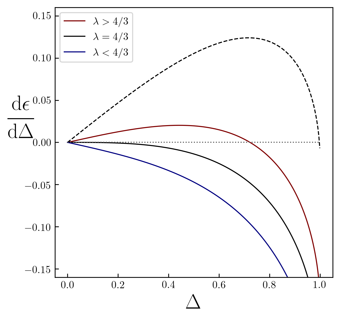
$$ \frac{\epsilon}{\epsilon_0} = \frac{3}{5} \frac{1}{2} \left[ (1+\Delta)^{5/3} + (1-\Delta)^{5/3} \right] + \frac{\lambda}{4} (1-\Delta^2)\,.$$

The minimum of the energy, for small $\lambda$, corresponds to the paramagnetic phase with $\Delta=0$. However, for larger values of $\lambda$, a minimum at finite $\Delta$ is possible. Indeed, in the figure below we show that the zero of the derivative,

$$ \frac{\D \epsilon}{\D \Delta} = 0$$

occurs at $0< \Delta < 1$ for $4/3 < \lambda < 2^{2/3}$ (for $\lambda > 2^{2/3}$ there is no solution). The critical value,

$$\alpha_c = \frac{4}{3} (3\pi^2)^{2/3} \frac{\hbar^2}{2m} n^{-1/3}$$

is the threshold for the appearance of a ferromagnetic phase.

Stability of the paramagnetic state in the Stoner model. When the interaction strength is $\lambda > 4/3$ the paramagnetic state is unstable and a spontaneous magnetization arise. The dashed line $\lambda= 2^{2/3}$ corresponds to a complete spin up phase.

A simple way to explore the transition is to expand the energy in powers of $\Delta$. Using sympy, it is easy to compute the power series:

from sympy import *
x = symbols('x', real=True)
a = symbols('a', real=True, positive=True)
series((1 + x)**a, x, n = 5)

which gives,

$$1 + ax + x^{2} \left(\frac{a^{2}}{2} - \frac{a}{2}\right) + x^{3} \left(\frac{a^{3}}{6} - \frac{a^{2}}{2} + \frac{a}{3}\right) + x^{4} \left(\frac{a^{4}}{24} - \frac{a^{3}}{4} + \frac{11 a^{2}}{24} - \frac{a}{4}\right) + O\big(x^{5}\big)$$

or, applied to our formula, up to second order:

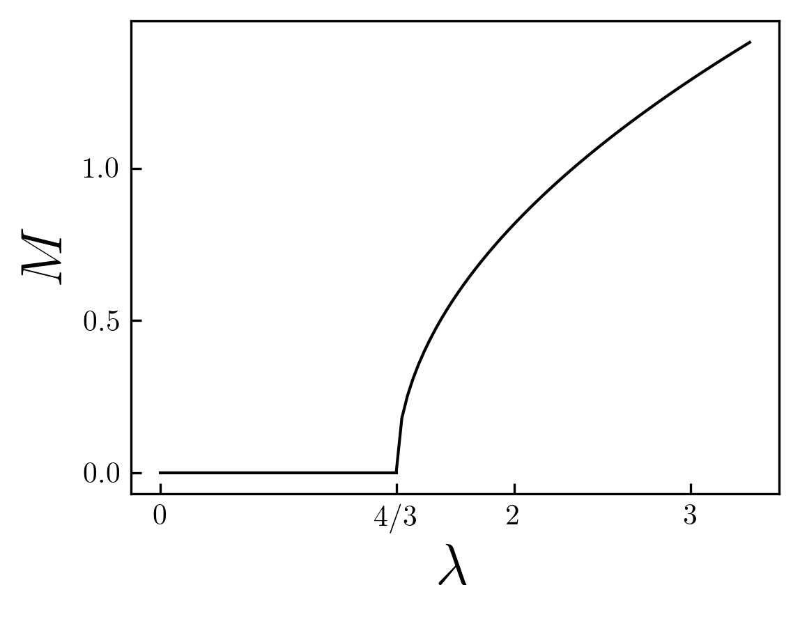
$$ \frac{\epsilon}{\epsilon_0} \approx \frac{3}{5} + \left( 1 - \frac{3\lambda}{4} \right) \frac{\Delta^2}{3}$$

showing that the second order term change sign precisely at $\lambda = 4/3$. Adding the fourth order term in the energy series expansion, one may find that the magnetization $M\sim\Delta$ is proportional to,

$$M\sim (\lambda - \lambda_c)^{1/2}\,.$$

This is analogous to the behavior of the mean field temperature dependence of the magnetization in the ising model; however, here the ferromagnetic transition is triggered by the interactions.

Qualitative behavior of the magnetization $M$ as a function of the coulomb repulsive interaction $\lambda$: above $\lambda_c=4/3$ the magnetization grows as a power low in $(\lambda-\lambda_c)^{1/2}$.