$\newcommand{\I}{\mathrm{i}} \newcommand{\E}{\mathrm{e}} \newcommand{\D}{\mathop{}\!\mathrm{d}} \newcommand{\Di}[1]{\mathop{}\!\mathrm{d}#1\,} \newcommand{\Dd}[1]{\frac{\mathop{}\!\mathrm{d}}{\mathop{}\!\mathrm{d}#1}} \newcommand{\bra}[1]{\langle{#1}|} \newcommand{\ket}[1]{|{#1}\rangle} \newcommand{\braket}[1]{\langle{#1}\rangle} \newcommand{\bbraket}[1]{\langle\!\langle{#1}\rangle\!\rangle}$

Lectures on statistical mechanics.

Molecular interactions

The pressure of the ideal gas is essentially due to the entropy, which leads to an effective repulsive force. In real gases molecular attractive and repulsive interactions do also contribute to the pressure, modifying the equation of state. The origin of molecular forces is mainly electrostatic: coulomb forces between the positively charged nucleus and negatively charged orbital electrons are eventually responsible for the large variety of molecular interactions not only in rarefied media but also in condensed matter. Examples are ionic and covalent bonds, van der Waals forces, long range dipole interactions, molecule-solvent or colloidal interactions.¹ Other forces include exchange (related to the identity of particles) and spin interactions that are generally important at very short distances, of the order of the separation of atoms in a crystal structure. In neutral gases, the interactions are of the van der Waals type; their strength is controlled by the polarizability of the molecules, they are repulsive at short distances and attractive at long distances. A rather universal interaction energy is given by the Lennard-Jones potential,

$$w(r) = \frac{A}{r^{12}} - \frac{B}{r^6} = 4\epsilon \left[ \left(\frac{r_0}{r}\right)^{12} - \left(\frac{r_0}{r}\right)^{6} \right]\,,$$

where $r$ is the distance between the atoms; the power $6$ of the attractive part is the London dispersion force between two induced dipoles, and the repulsive exponent is phenomenological. The order of magnitude of the coefficients is $A=10^{-134} \, \mathrm{J\, m^{12}}$ and $B=10^{-77} \, \mathrm{J\, m^{6}}$; this gives a repulsive core size $r_0 \approx 0.3\, \mathrm{nm}$, and a binding energy $\epsilon \approx 16\,\mathrm{meV}$.

We may distinguish short and long range interactions by considering the family of potentials,

$$w(r) = -\frac{C}{r^n} \,, \quad R > r_0\,,$$

parametrized by $n$, a positive number, where $C$ is a dimensional constant and $r_0$ the short distance cutoff (the atom “size”). The total energy of interaction of one atom with all the others, assuming a uniform distribution of density $\rho$, is

$$E = \int_{r_0}^L \D r\, 4\pi r^2\, w(r) = -4\pi C \rho \int_{r_0}^L \D r \, r^{2-n} = -\frac{4\pi C \rho}{(n-3) r_0^{n-3}} \left[ 1 - \left(\frac{r_0}{L}\right)^{n-3} \right]\,,$$

from which we deduce that if $n\le 3$ the total size of the system $L$ must be taken into account $E = E(L)$, while in the other case $n>3$, the total energy is independent on $L$. Therefore, an interaction energy decreasing faster than $r^{-3}$ is short range, while for slower decrease, as in the important case of the unscreened coulomb potential $r^{-1}$, it is long range. Note that we computed the energy in three dimensions, the classification of the range of the interaction depends also on the dimensionality of the system (one may substitute $3 \rightarrow d$ by the dimension $d$ in the previous formulas). Note also that the limiting case $n=3$ is long range (the energy is logarithmic in $L$).

The role of interactions is fundamental in determining the wealth of properties of materials and their transformations. Mechanical, magnetic, electrical and thermodynamical properties of matter depend on the interactions of its constituents, notably their diluted or condensed phases and the mechanisms of their transitions. The general framework to study the physical properties of matter is just the theory of statistical mechanics, we are left to compute, for a given model hamiltonian, and using appropriated approximations for each experimental situation, the (grand) partition function. Indeed, there is no universal method allowing the computation of the partition function, or equivalent statistical quantities; a large variety of methods, based on different assumptions, should be devised to solve specific problems. Here we study the cluster or virial expansion of the pressure in powers of density $N/V$ normalized to the size of the interacting atoms $v_0 \sim r_0^3$:

$$P \approx P_0 \left[1 + p_1 \frac{Nv_0}{V} + p_2 \left(\frac{Nv_0}{V}\right)^2 \ldots \right]$$

where $P_0$ is the ideal gas, and $B_2(T) = p_1 v_0$, $B_3(T) = p_2 v_0^2$, etc. are called the virial coefficients.² The idea is to find, as a first step, corrections to the ideal gas equation of state, and then, to extend the range of validity of the expansion using for instance, some type of resummation of a special kind of terms, or some phenomenological rule, in order to describe the transition of the gas to the liquid phase. In addition to this classical system, quantum states can also be studied using the same approach, to investigate the behavior of gases at very low temperatures. More explicitly, the grand partition function can be written as a series in the fugacity $z=\E^{\mu/T}$,

$$Z = \mathrm{Tr}\, \E^{-(H - \mu \hat{N})/T} = \sum_{N=0}^\infty \E^{\mu N/T}\, \mathrm{Tr}\, \E^{-H_N/T} = \sum_{N=0}^\infty z^N Z_N\,,$$

where $H_N$ is the hamiltonian of $N$ particles, and $Z_N = \mathrm{Tr}\,\E^{-H_N/T}$ is the “configuration” partition function. The thermodynamic potential,

$$\Phi = -T \ln Z = - T \ln \sum_{N=0}^\infty z^N Z_N$$

can also be written as a power series in the fugacity using the taylor expansion of the logarithm,

$$\Phi \sim \sum_N b_N z^N \,,$$

where $b_N = b_N(T,V)$ are so called “cluster” coefficients that should be determined at each order. Finally, using $N$ to eliminate the fugacity one eventually finds the searched coefficients $p_N$ in the expansion of the pressure.

Expansions of the form of $\Phi$ in powers of the fugacity or equivalently, $P = P(Nv_0/V)$ in powers of the density, are known in the theory of probability as a cumulant expansion.³

The virial expansion

We investigate the thermodynamics of a real gas whose hamiltonian contains two particle interactions $w$ depending on the distance between the gas atoms,

$$H_N = \sum_{n=1}^N \frac{p_n^2}{2m} + \sum_{n < m}^N w(|\boldsymbol x_n - \boldsymbol x_m|)\,,$$

where $\boldsymbol p_n$ and $\boldsymbol x_n$ are the momentum and position operators and $m$ the atom’s mass, and the sum is over the pairs of atoms (counted once and avoiding self-interaction, the number of terms is $N(N-1)/2$). The Lennard-Jones potential is a paradigmatic model of $w$. We shall discuss the classical case in parallel with the quantum one.

We implicitly assume that the interaction potential $w$ defines a characteristic length $r_0$, a short distance cutoff, associated to the atom’s volume $v_0 \sim r_0^3$, below which repulsion is strong. Another important property of $w$ is that it is an interaction aver all particle pairs; even if it is supposed to be short range, correlations between distant particles are possible by the superposition and propagation of near neighbors interactions (particles inside a sphere of radius the range of the interaction).

We start by writing the grand partition function in a form reminiscent to the exponential characteristic function in probability theory,

\begin{align} Z(T,\mu,V) & = \sum_{N=0}^\infty Z_N(T,V) z^N \nonumber\\ & = 1 + \sum_{N=1}^\infty \frac{M_N(T,V)}{N!} z^N\,, \end{align}

where we defined the “moments” $M_N$,

\begin{equation} M_N = N! \mathrm{Tr}\, \E^{-H_N/T} = N! \sum_n \E^{-E^{(N)}_n/T} \,, \end{equation}

where $E^{(N)}_n$ are the energy eigenvalues of the $N$-particles hamiltonian. It is useful to introduce, in the position representation, the nondimensional functions⁴ $W_N$ of the “configuration” $x = \boldsymbol x_1, \ldots, \boldsymbol x_N$:

\begin{equation} W_N(x) = N! \lambda^{3N} \braket{x|\E^{-H_N/T}|x} = N! \lambda^{3N} \sum_n\E^{-E^{(N)}_n/T} \phi^*_n(x)\phi_n(x)\,,\quad \,, \end{equation}

where $\lambda^2 = 2\pi \hbar/mT$ is the thermal length, such that,

\begin{equation} M_N = \int_{V^N} \prod_{n=1}^N \left(\frac{\D \boldsymbol x_n}{\lambda^3} \right) \, W_N(\boldsymbol x_1, \ldots, \boldsymbol x_N)\,, \end{equation}

where we used a properly symmetrized energy basis $\phi_n(x)$; $W_N$ represents the probability of the configuration $x$ in position space. The short range of molecular interactions ensures that in the extreme dilute limit, when the distances between the particles tend to infinity, $W_N \rightarrow 1$ EX.

The thermodynamic potential

$$\Phi(T,\mu,V) = -T \ln \left( 1 + \sum_{N = 1}^\infty \frac{M_N}{N!} z^N \right)\,,$$

can be expanded in terms of the “cumulants” $C_N=C_N(T,V)$:

\begin{equation} \Phi = -T \sum_{N=1}^\infty \frac{C_N}{N!} z^N\,. \end{equation}

In analogy with the moments, we define “Ursell functions” $U_N$ such that the cumulants $C_N$ correspond to the configuration integral of $U_N$,

\begin{equation} C_N = \int_{V^N} \prod_{n=1}^N \left(\frac{\D \boldsymbol x_n}{\lambda^3} \right) \,U_N(\boldsymbol x_1, \ldots, \boldsymbol x_N)\,. \end{equation}

The cumulants can readily be written in terms of the moments using the Bell polynomials:

$$C_N = \sum_{n=1}^N (-1)^{n-1} (n-1)! B_{N,n}(M_1,\ldots,M_{N-n+1})\,.$$

Therefore, for $N=1,2,3$,

\begin{align*} C_1 & = M_1 = 1\\ C_2 & = M_2 - M_1^2\\ C_3 & = M_3 - 3M_2 M_1 + M_1^3\,, \; \text{etc.} \end{align*}

The inverse formula, giving the moments as a combination of cumulants, reads,

$$M_N = \sum_{n=1}^N B_{N,n}(C_1,\ldots,C_{N-n+1})\,.$$

For $N=1,2,3$ we find,

\begin{align*} M_1 & = C_1 = 1 \\ M_2 & = C_2 + C_1^2 \\ M_3 & = C_3 + 3C_2 C_1 + 2C_1^3\,, \; \text{etc.} \end{align*}

The functions $U$ are related to the functions $W$ through the relation between their respective moments $M$ and cumulants $C$:

\begin{align*} W_1(\boldsymbol x_1) & = U_1(\boldsymbol x_1) = 1 \\ W_2(\boldsymbol x_1, \boldsymbol x_2) & = U_2(\boldsymbol x_1, \boldsymbol x_2) + U(\boldsymbol x_1) U(\boldsymbol x_2)\\ W_3(\boldsymbol x_1, \boldsymbol x_2, \boldsymbol x_3) & = U(\boldsymbol x_1, \boldsymbol x_2, \boldsymbol x_3) \\ & \qquad + U(\boldsymbol x_1, \boldsymbol x_2) U(\boldsymbol x_3) + U(\boldsymbol x_1, \boldsymbol x_3) U(\boldsymbol x_2) + U(\boldsymbol x_2, \boldsymbol x_3) U(\boldsymbol x_1) \\ & \qquad + U(\boldsymbol x_1) U(\boldsymbol x_2) U(\boldsymbol x_3) \,, \end{align*}

for $N = 1,2,3$. Indeed, the coefficients in the formula for the moments, the numbers $B_{N,n}$ give all the combinations of the position labels into clusters of $n$ particles, that once integrated out, give the same contribution to the corresponding moment. Therefore, their general expression contains the partitions $\mathcal{P}$ of the set $\mathcal{N} = \{1,\ldots,N\}$ and the blocks $s$ belonging to each partition,

$$W_N(\boldsymbol x_1,\ldots,\boldsymbol x_N) = \sum_{\mathcal{P} \in \mathcal{P}_N} \prod_{s \in \mathcal{P} } U_{|s|}(\boldsymbol x_{s})\,,$$

and the inverse formula,

$$U_N(\boldsymbol x_1,\ldots,\boldsymbol x_N) = \sum_{\mathcal{P} \in \mathcal{P}_N} \prod_{s \in \mathcal{P} } (-1)^{|\mathcal{P}|-1} (|\mathcal{P}|-1)! W_{|s|}(\boldsymbol x_{s}) \,,$$

where, explicitly, $\mathcal{P} = \{s_1,\ldots, s_K\}$ is a partition of the set $\mathcal{N}$ into disjoint subsets $s_k$, such that

$$\mathcal{N} = \bigcup_{k=1}^K s_k,\quad K = |\mathcal{P}|\,,$$

$\mathcal{P}_N$ is the set of all partitions of $\mathcal{N}$; $|\ldots|$ is the cardinal of the given set; $\boldsymbol x_s$ is the list of positions indexed by the subset $s$. Obviously, the indexes in $s$ are all different (self-interaction is absent). Then, the cumulants are specified by the irreducible correlations, interactions between a set of particles $s$ that cannot be decomposed into separated subsets of interacting particles (we can take this statement as a definition of a cluster).

Therefore, the grand partition function can be expanded in powers of the fugacity,

\begin{equation} \label{e:vThPot} \Phi(T,\mu,V) = -T \ln Z(T,\mu.V) = -T \frac{V}{\lambda^3} \sum_{N=1}^\infty b_N z^N\,, \end{equation}

using the cumulants of $N$ particles $C_N$, or equivalently the “cluster integrals”

\begin{equation} b_N(T,V) = \frac{\lambda^3}{VN!} C_N(T,V) \,. \end{equation}

The normalization of the cluster integrals is such that the limit

$$b_N(T) = \lim_{V\rightarrow\infty} b_N(T,V)\,,$$

is well defined.

The equation of the particle number of a diluted gas ($V \rightarrow \infty$, limit),

\begin{equation} \label{e:vPressure} \end{equation}

$$N = - \frac{\partial \Phi}{\partial \mu} = \frac{V}{\lambda^3} \sum_{N=1}^\infty N b_N(T) z^N\,, \quad b_N(T) = \lim_{V\rightarrow\infty} b_N(T,V)\,,$$

can be used to eliminate the fugacity by inverting the series, and replacing it into the thermodynamic potential $\eqref{e:vThPot}$, one obtains the equation of state $P=P(T,V,N)$. The final result is a series in the density,

\begin{equation} \label{e:vEqofState} P = \frac{NT}{V} \left(1 + B_2(T) \frac{N}{V} + B_3(T) \frac{N^2}{V^2} + \cdots \right) \end{equation}

whose coefficients are the “virial coefficients” $B_{N}(T)$. In particular, the second order virial coefficient is,

$$B_2(T) = -b_2(T) \lambda^3\,.$$

Note that at variance to the $b_N(T)$, the virial coefficients have dimensions of a power of a volume $B_N \sim v_0^{N-1}$.

As an example let us obtain the thermodynamics quantities of a system in terms of the second cluster coefficient $b_2$. We start with the number of particles as a function of the fugacity,

$$N = \frac{V}{\lambda^3}(z + 2 b_2 z^2)$$

which gives by inversion of the series, the fugacity in powers of $N/V$:

$$z = \frac{\lambda^3}{V} \left( 1 - 2 b_2\frac{\lambda^3 N}{V} \right)\,.$$

Replacing this last expansion into $\Phi$ one obtains the equation of state (valid to second order in the density),

$$PV = NT \left( 1 - b_2 \frac{\lambda^3N}{V} \right)\,.$$

We note that the virial coefficient $B_2(T)=-b_2(T) \lambda^3$. It is also useful to write the free energy EX,

$$F(T,V,N) = -NT \ln \frac{\E V}{\lambda^3N} - \frac{N^2T}{V} \lambda^3b_2\,,$$

from which one may obtain the entropy, thermodynamic energy and heat capacity at constant volume. (Of course, the first term is the ideal gas free energy.) For instance, the energy is given by,

$$E = \frac{3NT}{2} + \frac{3NT}{2} \frac{N\lambda^3}{V} \left( \frac{2T}{3} \frac{\D b_2}{\D T} - b_2 \right)\,.$$

All the above formulas are equally valid irrespective of the statistics. The specificity of the statistics appears as a property of the states $\ket{\boldsymbol x_1,\ldots,\boldsymbol x_N}$ symmetry: symmetric or antisymmetric for bosons or fermions, without restrictions for the Boltzmann statistics. We shall discuss first the classical case, in which the hamiltonian reduces to a phase-space function.

Mayer classical cluster expansion

The classical expression for $M_N$, taking into account that $W_N \sim \E^{-w/T}$ and that the momentum integrations are included in the expression of $Z_1$, can be written as a product of pair interactions using the Mayer functions $f_{mn}$

$$M_N = \int_{V^N} \prod_{n=1}^N \frac{\D \boldsymbol x_n}{\lambda^3} \, W_N \,,\quad W_N = \prod_{m<n}^N (1+f_{mn})\,,$$

where,

$$f_{mn} = \exp\big[-w(|\boldsymbol x_m - \boldsymbol x_n)/T \big] - 1\,.$$

These functions have the desirable properties of being for small distances between the two atoms $m$ and $n$, $f(r) \rightarrow -1$, and for large distances, $f(r) \rightarrow 0$ (contrary to the simple $W$ that is finite at large distances, making its integral divergent with the system’s size).

Developing the product, we observe that the functions $W_N$ contains terms without pairings, with the pairing of two particles $\sim f$, three particles $\sim ff$ up to $N$ particles $ff\ldots f$ (the length of this last term is $N(N-1)/2$, the total number of pairs). A graphical visualization is useful: representing a particle by a node, and an interaction $f_{mn}$ by a link between nodes $m$ and $n$, we can associate a graph of nodes and links to each different product $f\ldots f$:

Three particles diagrams. The first graph contains one two-particle cluster and one unlinked particle, it corresponds to $f_{12}$; the two other graphs are connected: $f_{12}f_{23}$ and $f_{12}f_{23}f_{13}$, respectively. The second diagram is “reducible” (it decomposes into lower order clusters): if one cuts a link a it becomes disconnected. The third diagram is “irreducible”: cutting a link do not disconnect the cluster. A cluster is a set of linked nodes.

The above figure is part of the function $W_3$:

$$W_3 = 1 + f_{12} + f_{13} + f_{23} + f_{12}f_{23} + f_{13}f_{23} + f_{12}f_{13} + f_{12}f_{23}f_{13}\,,$$

which corresponds to the sum of all graphs with three particles. The $U$ functions are given by the sum of the connected graphs:

\begin{align*} U_1 & = 1 \\ U_2 & = f_{12} \\ U_3 & = f_{12}f_{23} + f_{13}f_{23} + f_{12}f_{13} + f_{12}f_{23}f_{13}\,, \end{align*}

here, the clusters of three particles.

Qualitatively, we can say that the partition function can be decomposed in a sum of unrestricted graphs, while the cumulants are a sum of connected graphs,

$$Z\sim \sum\; \text{graphs} \sim \exp{\big( \text{connected graphs} \big)} \sim \exp\left( -\frac{\Phi}{T} \right)\,.$$

Let us apply the above formalist to the computation of the firsts cumulants $C_N$ in the classical case. The general form of the cumulants is,

$$C_N = \int_{V^N} \frac{\D \boldsymbol x_1 \ldots \boldsymbol x_N}{\lambda^{3N}} \sum\left( \text{connected graphs}\right) \sim \int f_{12} f_{13} \ldots f_{N-1,N} + \ldots$$

They are dimensionless, and have the important property that they converge in the thermodynamic limit,

$$\lim_{V\rightarrow\infty} \frac{\lambda^3}{VN!} C_N = \lim_{V \rightarrow \infty} b_N(T,V) \equiv b(T)\,,$$

where we defined the $b(T)$ as the limit $V\rightarrow\infty$ of the cluster integrals, which are useful in the case of a dilute gas, to obtain the virial expansion of the pressure in powers of the density (or specific volume).

We start with $b_2 = \lambda^3 C_2/2V$,

$$b_2 = \frac{1}{2V\lambda^3} \int_{V^2} \D \boldsymbol x_1 \D \boldsymbol x_2 \, U_2(\boldsymbol x_1, \boldsymbol x_2) = \frac{1}{2\lambda^3} \int_0^\infty 4\pi r^2 \D r\, f_{12}(r) = -\frac{B_2(T)}{\lambda^3}\,,$$

where we used the isotropy of the interaction, which depends only on the distance $r=|\boldsymbol x_1 - \boldsymbol x_2|$. The last equality introduces the second virial coefficient $B_2$ of the pressure expansion $\eqref{e:vPressure}$:

$$B_2(T) = \frac{1}{2} \int_0^\infty 4\pi r^2 \D r\, \left(1 - \E^{-w(r)/T} \right)\,,$$

for particles interacting through a spherical symmetric potential $w(r)$.

van der Waals equation of state

The simplest case is the rigid sphere interaction, consisting in a hard core $w=\infty$ if $r<r_0$, and no interaction for larger distances. In this case the evaluation of the integral is trivial,

$$\int_0^\infty \D r\, r^2 (\E^{-w(r)/T} - 1) = - \int_0^{r_0} \D r\, r^2 = - \frac{r_0^3}{3}\,,$$

and the cumulant,

$$b_2 = - \frac{v_0}{2\lambda^3},\quad v_0 = \frac{4}{3}\pi r_0^3\,.$$

Putting this result in the equation for the thermodynamic potential,

$$\Phi = -PV = -T \frac{V}{\lambda^3} z\left(1 - \frac{v_0 }{\lambda^3} \frac{z}{2}\right)\,,$$

we can derive the equation of state eliminating the fugacity. The number of particles is given by the logarithmic derivative of $\Phi$ with respect to the fugacity,

$$N = \frac{V}{\lambda^3}\left(z - \frac{v_0}{\lambda^3} z^2 \right)\,.$$

Using $z \approx \lambda^3 (N/V) = \lambda^3 n$, one obtains

$$PV = NT (1 + b n), \quad b = \frac{v_0}{2}\,,$$

where $b = -VC_2/2=B_2$ is the second virial coefficient, in this case independent of the temperature. We found that the presence of a repulsion force between atoms at short distances leads to a correction to the ideal gas equation of state that essentially reducing the available volume $V \rightarrow V(1-bn)$. We can rewrite the correction in a more explicit form,

$$PV = N T (1 + bn) = NT \frac{1}{1-bn}\,,$$

(to the same order) or

$$P(V-bN) = NT\,,$$

where the coefficient $b$ appears clearly as an excluded volume per atom. In order to find this effect we used a method of resummation of one particular class of terms in the virial expansion, whose validity is mostly phenomenological.

In real (neutral) gases a long distance attractive force is present, due to the induced polarizability of the atoms,

$$w(r) \sim -\epsilon(r_0/r)^6\,,$$

as in the Lennard-Jones potential. This attractive effect also leads to a modification of the pressure, purely repulsive and entropic in an ideal gas. Its contribution to the second cumulant is,

\begin{align*} b_2 & = \frac{4\pi}{2\lambda^3} \int_0^\infty r^2 \D r\, \left( \E^{-w(r)/T} - 1 \right) \\ & \approx -\frac{2\pi}{\lambda^3} \int_0^{r_0} r^2 \D r + \frac{2\pi}{\lambda^3} \int_{r_0}^\infty r^2 \D r \left( \E^{\epsilon r_0^6/r^6 T} - 1 \right)\,, \end{align*}

where we split the integral into a hard core part and an attractive force part. The second integral is readily evaluated for $\epsilon < T$ as a power series (high temperature expansion, valid in the gas phase) EX,

\begin{align*} b_2 & = -\frac{v_0}{2\lambda^3} + \frac{v_0}{2\lambda^3} \sum_{n=1}^\infty \frac{1}{2n-1} \left(\frac{\epsilon}{T}\right)^n \\ & \approx \frac{v_0}{2\lambda^3} \left(-1 + \frac{\epsilon}{T} \right)\,, \end{align*}

(note that the two contributions have opposite signs). Keeping the first term in the temperature expansion, we obtain the second virial coefficient

$$B_2(T) = \frac{v_0}{2} \left(1 - \frac{\epsilon}{T} \right)$$

from which we get the van der Waals equation of state,

$$\left(P + \frac{N^2 a}{V^2} \right) (V-Nb) = NT,$$

where the (phenomenological) parameters are related, in the present model, to the parameters of the microscopic potential by $b=v_0/2$ and $a=v_0 \epsilon/2$. The temperature dependent part of the correction is due to the attractive forces between atoms at long distances, which results in a weakening of the pressure the gas exerts to the exterior (e.g. enclosing walls).

Interacting fermi gas

It is possible, using magneto-optical traps, to confine a gas of fermions at temperatures of the order of the fermi temperature (e.g Li$^6$ at $T_F\approx 8\,\mu\mathrm{K}$).⁵ The experimental setup allow to tune the strength and range of the interaction using an external magnetic field $B \sim 10\!-\!\!100 \, \mathrm{mT}$, arround the Feshbach resonance, and therefore to explore the physics of strongly interacting quantum systems. We shall investigate the thermodynamic properties of the fermi gas near the resonance, using a virial expansion to second order. The degeneracy of the gas and the strong van der Waals interactions impose a quantum calculation.

The thermodynamic potential, expanded to quadratic terms in the fugacity $z=\E^{\mu/T}$, is

$$\Phi = - \frac{TV}{\lambda^3}(z + b_2 z^2)$$

where $b_2$ is the second cluster coefficient,

$$b_2 = \frac{\lambda^3}{2V} C_2 = \frac{\lambda^3}{2V} (M_2 - M_1^2)\,, \quad M_2 = 2\sum_n \E^{-E^{(2)}_n/T}\,. $$

The spectrum of the two body hamiltonian depends on the total momentum eigenvalues $P$ and the quantum numbers $n$ of the relative motion eigenfunctions. It can be written,

$$E^{(2)}(P,n) = \frac{P^2}{4m} + \epsilon_n$$

where $2m$ is the total mass and the energy levels are obtained from the solution of the reduced Schrödinger equation,

$$\left[- \frac{\hbar^2}{m}\nabla^2 + w(r) \right]\phi_n(\boldsymbol x) = \epsilon_n \phi_n(\boldsymbol x)\,,$$

where $\boldsymbol x = \boldsymbol x_1 - \boldsymbol x_2$ and $r = |\boldsymbol x|$, $m/2 = m^2/2m$ is the reduced mass and $\phi_n$ are the eigenfunction of the energy state $n$ (discrete or continuous). In the absence of interaction, the free particle energies are labelled by the wavevector $k_n$,

$$\epsilon^{(0)}_n = \frac{\hbar^2 k_n^2}{m}\,,$$

where the index $(0)$ refers to the noninteracting system $w\rightarrow0$, we will use as a reference.

The contribution of the center of mass motion to the second moment can be readily computed,

$$\sum_P \E^{-P^2/4mT} = \frac{V}{(2\pi\hbar)^3} \int_0^\infty 4\pi P^2 \D P\, \E^{-P^2/4mT} = 2^{3/2} \frac{V}{\lambda^3}$$

which gives,

$$M_2 = 2^{5/2} \frac{V}{\lambda^3} \sum_n \E^{-\epsilon_n/T}\,.$$

The shift of the second cluster coefficient $\Delta b$ with respect to the noninteracting case, is therefore,

$$\Delta b = b_2 - b_2^{(0)} = 2^{3/2} \sum_n \left( \E^{-\epsilon_n/T} - \E^{-\epsilon_n^{(0)}/T} \right)\,.$$

The coefficient $b_n^{(0)}$ are, for free fermions EX,

$$b_n^{(0)} = - \frac{(-1)^n}{n^{5/2}}\,.$$

(Note that “free” fermions, as well as bosons, are in fact correlated by the symmetry constraint on their quantum state, i.e. particles’ identity.)

For a diluted system, like a gas, the particle interactions can be well described in the framework of scattering theory:⁶ interactions are essentially due to particle collisions. The interacting spectrum $\epsilon_n$ contains, in general, a set of bound states $-\epsilon_B>0$ and a continuum spectrum $\hbar^2 k^2/2m$ ($k\in \mathbb{R}$). Note however that bound states in the continuum are also possible, like in the case of diffusion resonances (Fano, Feshbach). The discrete part of the spectrum appears only in the interaction part of the thermodynamic potential, while the continuum spectrum appears in both $b_2$ and $b_2^{(0)}$. The asymptotic form of the radial wavefunction $u(r)$, in the partial wave decomposition of $\phi(\boldsymbol x) \sim u(r) Y_{lm}(\theta,\varphi)$, is

$$u(r) \sim \frac{\text{const.}}{r} \sin(kr - \pi l/2 + \delta_l)\,,$$

where $\delta_l(k)$ is the scattering phase shift of the $l$-wave (angular momentum). Inside a volume of radius $R$, the boundary condition imposes,

$$kR - \pi l / 2 + \delta_l = n\pi, \quad n \in \mathbb{N}\,.$$

For a large $R$ the difference between consecutive $k$ is small, to first order we have,

$$dn = \frac{R}{\pi} \D k + \frac{1}{\pi} \frac{\D \delta_l}{\D k} \D k \,,$$

from which we may define $g(k)$ the density of states of wavenumber $k$

$$g(k) = \frac{1}{\pi} \sum_l (2l+1) \left( R + \frac{\D \delta_l}{\D k} \right)\,,$$

where the sum is over all the two fermions angular momentum states: $l=1,3,\ldots \in 2\mathbb{N}+1$ for fermions, and $l=2,4,\ldots \in 2\mathbb{N}$ for bosons. Therefore, using the replacement,

$$\sum_n \ldots \rightarrow \int_0^\infty \D k g(k) \ldots$$

in the formula of $\Delta b$, we obtain the Beth-Uhlenbeck (1937) formula,

$$ \Delta b = 2^{3/2} \sum_B \E^{-\epsilon_B/T} + \frac{2^{3/2}}{\pi} \sum_{l \in 2 \mathbb{N} + 1} (2l+1) \int_0^\infty \D k \, \E^{-\lambda^2 k^2/2\pi} \frac{\D \delta_l(k)}{\D k}$$

where the term proportional to $R$ cancels with the noninteracting term ($\delta_l \rightarrow 0$). The first term is the contribution of the bound states, and the second one, of the scattering states (with the free states contribution substracted). This is a general formula that can also be applied to bosons if the sum is effected on even $l$ orbital numbers. Using the value of the second cluster coefficient $b_2 = b_2^{(0)} + \Delta b$, we can calculate the thermodynamics of the system.

Now, we apply the Beth-Uhlenbeck formula to the case of a gas of fermions near the Feshbach resonance. As we said before, one important property of the Feshbach resonance is that the diffusion length $a$, and hence the type of interaction (from attractive to repulsive), can be modified by an applied magnetic field $B$:

$$a(B) = a_0 - \frac{a_0}{\mu_\mathrm{B}}\frac{\Delta}{B-B_0}\,,$$

($\mu_\mathrm{B}$ is a magnetic moment) where $a_0$ is the “background channel” diffusion length (see the figure), and $B_0$ the resonant field.

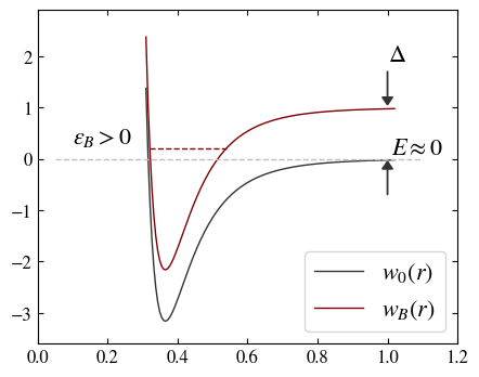
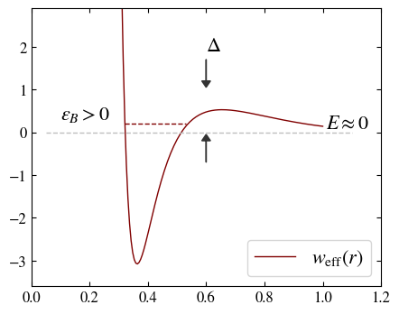
Feshbach resonance mechanism. (first) Two particles having different magnetic moments (like a proton and a neutron) collide (open channel $E\approx 0$) at low energy; the pair of particles support a bound state (closed channel, like a deuterium state) whose energy is slightly positive ($\epsilon_B >0$, is a metastable state). (second) Near the resonance, the scattering process can be described by an effective potential with a metastable bound state. For a gas of strongly interacting fermions, the Feshbach resonance is a many-body effect that change the macroscopic behavior of the system.⁷

The presence of the resonance simplifies the analysis, because it is not necessary to completely solve the two body problem to find the behavior of the phase shift $\delta_l$. First, we consider the low energy scattering s-wave limit ($l=0$), which is the relevant one in experiments; the phase shift can be parametrized by the diffusion length $a$ and the interaction range length $r_0$:

$$k \cot \delta_0(k) = -\frac{1}{a} + \frac{r_0}{2} k^2\,,$$

which leads to,

$$\frac{\D \delta_0}{\D k} = -a\frac{1 + ar_0 k^2/2}{(1 - ar_0 k^2/2)^2 + a^2k^2}\,.$$

Replacing this derivative into the integral, and changing to the variable $x = |a|k$, the integral becomes,

$$I = -\mathrm{sgn}(a) \int_0^\infty \D x \, \frac{1 + \alpha x^2}{(1- \alpha x^2)^2 + x^2} \E^{-\beta x^2} \,, \quad \alpha = \frac{r_0}{2a},\; \beta = \frac{\lambda^2}{2\pi a^2} \,.$$

The virial coefficient is then given by,

\begin{equation} \label{Ho} \Delta b_2(T) = 2^{3/2}\E^{-\epsilon_B/T} + \frac{2^{3/2}}{\pi} I \,. \end{equation}

Near the resonance $\alpha \ll 1$, which allows an asymptotic calculation of the integral. To first order in $\alpha$, we find,

$$I \approx I^{(0)} + I^{(1)}\,,$$

with

$$I^{(0)} = -\mathrm{sgn}(a) \frac{\pi}{2} \E^{\lambda^2/2\pi a^2} \mathrm{erfc}\left(\frac{\lambda}{\sqrt{2\pi}|a|}\right)\,, $$

and

$$I^{(1)} = -\frac{\pi}{2^{3/2}} \frac{r_0}{\lambda} \left(1 - \frac{\lambda^2}{\pi a^2} \right) - \frac{r_0}{4|a|} \frac{\lambda^2}{a^2} \E^{\lambda^2/2\pi a^2} \mathrm{erfc}\left(\frac{\lambda}{\sqrt{2\pi}|a|}\right)\,. $$

Taking into account the first correction in $r_0$, we have,

$$I \approx -\frac{\pi \mathrm{sgn}(a)}{2} + \frac{\lambda}{\sqrt{2}a} - \frac{\pi r_0}{2^{3/2}\lambda}\,,$$

where we used the approximation $\mathrm{erfc}(x) \approx 1- 2x/\sqrt{\pi}$, which leads to a virial coefficient,

$$\Delta b_2 = 2^{3/2} \E^{-\epsilon_B/T} - \sqrt{2} \mathrm{sgn}(a) + \frac{4}{\sqrt{\pi} a k_F} \sqrt{\frac{T_F}{T}} - \frac{r_0k_F}{2\sqrt{\pi}} \sqrt{\frac{T}{T_F}}\,, $$

where we used the notation $T_F = \hbar^2 k_F^2/2m$, for the fermi temperature and wavenumber. Using the experimental data, this expression gives the order of magnitude of the corrections to the thermodynamic quantities due to the particles interactions.

A comparison of the virial expansion of the interaction energy,⁸

$$E_{\text{int}} = \frac{3NT}{2} \frac{N\lambda^3}{V} \left( \frac{2T}{3} \frac{\D b_2(T)}{\D T} - b_2(T) \right)\,,$$

where $b_2$ is given by ($\ref{Ho}$), gives an excellent qualitative agreement with the experiments of Bourdel et al.⁵.

Notes

Israelachvili, J. N., Intermolecular and Surface Forces (2011). ↩
Landau, L.D., and Lifshitz, E. M., Statistical Physics (1980). ↩
Shiryaev, A. N., Probability (1996). ↩
Kahn, B. and Uhlenbeck, G. E., On the theory of condensation, Physica 5, 399 (1938) ↩
Bourdel, T., Cubizolles, J., Khaykovich, L., Magalhães, K. M. F., Kokkelmans, S. J. J. M. F., Shlyapnikov, G. V., and Salomon, C., Measurement of the interaction energy near a Feshbach resonance in a $^6$Li fermi gas, Phys. Rev. Lett. 91, 020402 (2002). ↩↩
Le Bellac, M., Physique quantique (2007). ↩
Chin, Cheng and Grimm, R., Julienne, P., and Tiesinga, E., Feshbach resonances in ultracold gases, Rev. Mod. Phys. 82, 1225 (2010). ↩
Ho, Tin-Lun, and Mueller, E. J., High Temperature Expansion Applied to Fermions near Feshbach Resonance, Phys. Rev. Lett. 92, 160404 (2004). ↩