Classical dynamical systems

$\newcommand{\I}{\mathrm{i}} \newcommand{\E}{\mathrm{e}} \newcommand{\D}{\mathop{}\!\mathrm{d}}$

»chaos »map »hamiltonian systems »plasmas

Stability

A continuous time dynamical system $x(t)$ is governed by a differential equation

$$\dot{x} = F_a(x,t)$$

where the law $F$, which determines the evolution of $x$, depends in general on a set of parameters $a$. Therefore, the evolution of the dynamical variable, solution of this equation, will depend on the inital condition $x_0$ together with the set $a$: $x=x_a(t; x_0)$. Changes in the values of $a$ may change the qualitative behavior of $x(t)$. For instance, the topology of the family $x_a(t; x_0)$ for a set of initial conditions, may change at some specific value $a=a_*$. The topology of the family of trajectories, which is similar to a vector field, is largely determined by the fixed points $X$,

$$F_a(x, t) = 0,\quad x=X_n,\; n=0,1,\ldots$$

and the behavior of the trajectories in the neighborhood of these fixed point. For instance, a fixed point $X_0$ is say to be stable if neighboring trajectories stick near $X_0$ for long times, if initially they were near $X_0$ (Lyapounov stability). One useful method to determine the stability of a fixed point consists in the linearization of the evolution equation around the fixed point, $x=X+\Delta x$:

$$\Delta\dot{x} = \left.\frac{\partial F}{\partial x}\right|_X\,\Delta x = M(X) \Delta X\,,$$

which, according to the values of the complex eigenvalues $\lambda$ of the matrix $M(X)$, leads to the classification:

$X$ is stable if $\mathrm{Re}\, \lambda < 0$, otherwise, if $\mathrm{Re} \, \lambda > 0$, there exists a solution with $x(t) \rightarrow \infty$ for $t \rightarrow \infty$.
for purely imaginary eigenvalues $\mathrm{Re}\, \lambda = 0$ (conjugate pairs), neighboring trajectories of $X$, are periodic.

A stable fix point is the simplest attractor, an invariant subset of the phase space resulting from the asymtotic contraction of trajectories initially occupying a large volume of the phase space.

Example: Kelvin-Helmholtz instability


Visualization of the flow around a plate moving in a fluid

A tangential discontinuity of the velocity field $\boldsymbol{v}$ in a potential two dimensional flow is characterized by the vorticity density distribution, the jump in the velocity $\kappa = v_\parallel^{(+)} - v_\parallel^{(-)}$ parallel to the discontinuity line:

$$\kappa(s,t) \D s = \D\Gamma(s),\quad \frac{\D \Gamma}{\D t} = 0$$

where $\Gamma(s)$ is the circulation of the velocity field at the point $s$ of the discontinuity line $\ell$. Moreover, in an ideal fluid, the circulation is conserved. The velocity field satisfies, outside the vortex line $\ell$, Poisson equation

$$\boldsymbol v = \nabla \phi,\quad \nabla^2 \phi = 0,\quad (x,y) \not\in \ell$$

Using a representation of the $(x,y)$ plane in terms of the complex variable $z = x + \I y$, the Biot-Savart equation reads,

$$v_x - \I v_y = \bar{v} = \frac{1}{2\pi \I} \int_\ell \D s \frac{\kappa(s,t)}{z - Z(s,t)}$$

where the line $z=Z$, is parametrized by $Z = Z(s,t)$, and $v$ is the complex velocity. From potential theory, the velocity field at the discontinuity is given by the mean $V= (v^{(+)}+v^{(-)})/2$:

$$V = \frac{\D \overline{Z(\Gamma,t)}}{\D t} = \mathrm{PV} \int \frac{\D \Gamma'}{2\pi \I} \frac{1}{Z(\Gamma,t) - Z(\Gamma',t)}$$

known as the Birkhoff-Rott equation.

A fixed point $\D \bar{Z}/\D t = 0$ is simply given by the straight line $Z(\Gamma,t) = \Gamma/U$, if the vorticity distribution is uniform and $U=v_\parallel^{(+)} - v_\parallel^{(-)}$ is the tangential velocity jump. A periodic perturbation $\Delta Z$ of the stationary solution, can be decomposed in fourier modes of wavenumber $k = 2\pi n/L$ (we take units such that $U=1$ and $L=1$):

$$Z(\Gamma,t) = \Gamma + \sum_{n\in \mathbb{Z}} a_n(t)\, \E^{\I 2\pi n \Gamma} = \Gamma + \Delta Z(\Gamma,t)\,,$$

in these units, the periodicity is $L=1$, $Z(\Gamma + 1, t) = Z(\Gamma,t) + 1$. Inserting the perturbation into the Birkhoff-Rott equation, and linearizing one obtains,

$$\frac{\D \overline{\Delta Z}}{\D t} = -\mathrm{PV} \int \frac{\D \Gamma'}{2\pi \I} \frac{\Delta Z(\Gamma,t) - \Delta Z(\Gamma',t)}{|\Gamma - \Gamma'|^2}$$

or, using $u = \Gamma'-\Gamma$,

$$\sum_n \frac{\D \bar{a}_n}{\D t} \E^{-\I 2\pi n \Gamma} = -\sum_n a_n \E^{\I 2\pi n \Gamma}\, \mathrm{PV}\int_{-\infty}^{\infty} \frac{\D u}{2\pi\I} \frac{1-\E^{\I 2\pi n u}}{u^2}\,.$$

The principal value integral gives $\pi |n|/\I$, therefore, equating similar terms one obtains,

$$\frac{\D \bar{a}_n}{\D t} = \I\pi |n| a_{-n}$$

which leads, after integration, to an exponentially growing function, with growth rate $\sigma$ proportional to the perturbation wavenumber:

$$a_n(t) = a_n(0) \E^{\sigma_n t}, \quad \sigma_n = \pi |n|\,.$$

In the original units, a perturbation of wavelength $L/n$ of a discontinuity $U$ grows in time with the rate

$$\sigma_n = \frac{\pi U}{L}|n|,\quad \sigma_k = U |k|/2\,.$$

Numerics

The dynamics of a periodic vortex line $z=x + i y = Z(s,t)$ is governed by the Birkhoff-Rott equation,

$$\frac{\partial}{\partial t}\bar{Z}(s,t)= \mathrm{PV} \int \frac{\D s'}{{2\I}} \kappa(s',t) \cot\left[\pi(Z(s,t)-Z(s',t))\right]\,,$$

where $\kappa(s,t)=|\partial Z/\partial \Gamma|^{-1}$ is the intensity, and a Coulomb like potential in $\ln \sin r$ instead of the $\ln r$ (distance $r$), adapted to the two dimensional domain with periodic boundary conditions is the $x$ direction.

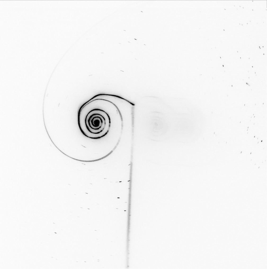
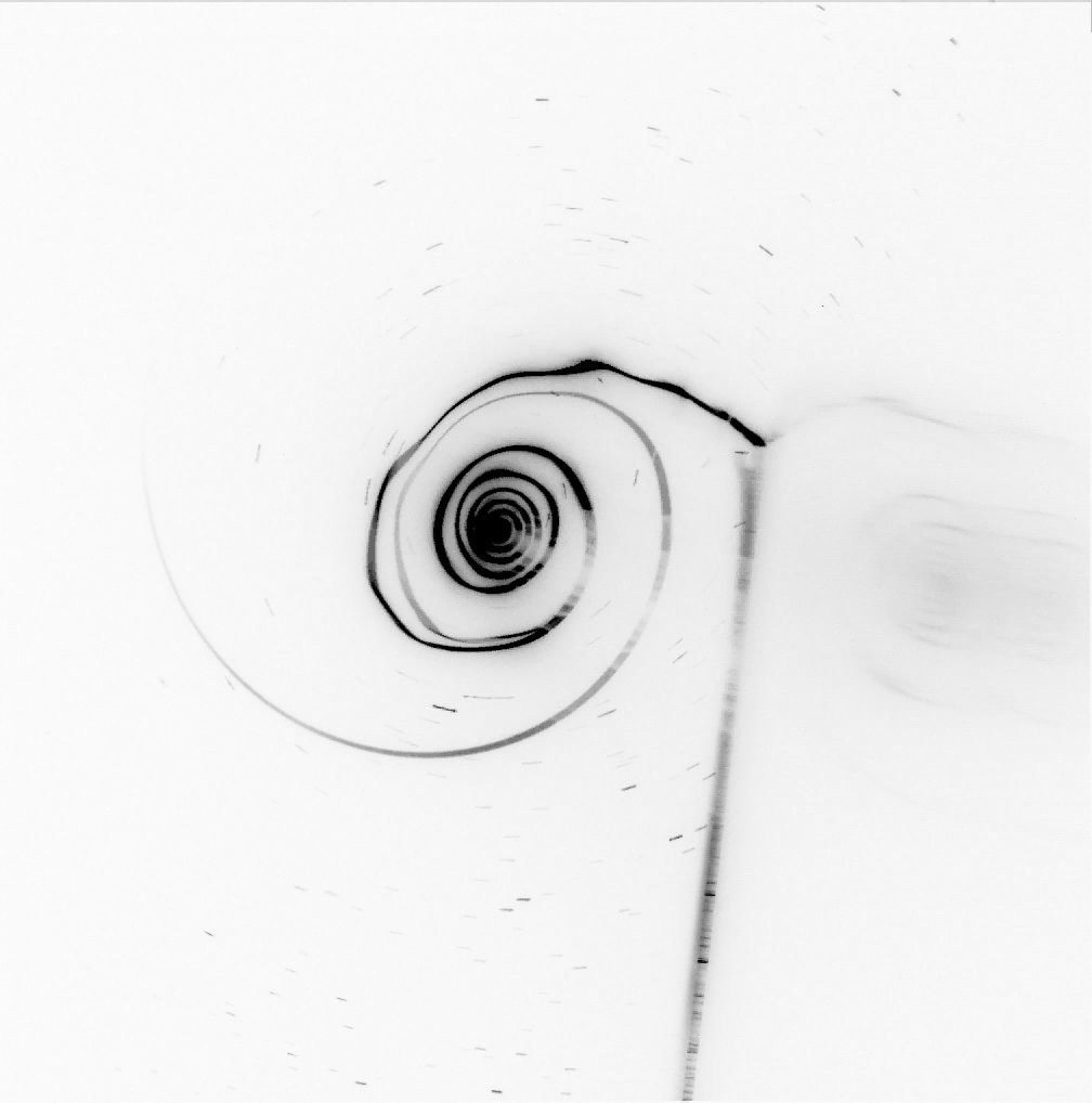
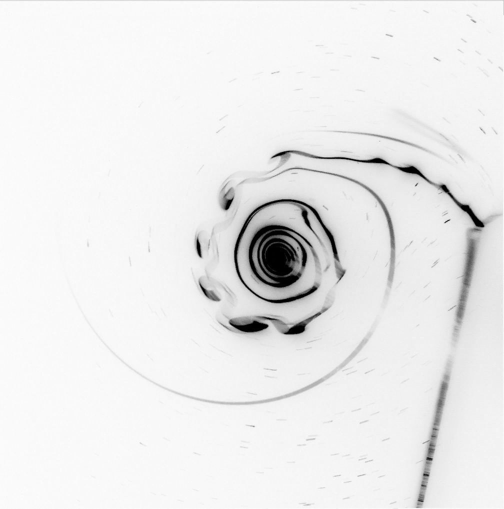
The tangential discontinuity can be approximated by a one dimensional array of point vortices interacting with a $\ln \sin \pi r_{ij}$ type potential, where $r_{ij}$ is the separation between pairs $(i,j)$ of the point vortices. The motion of a given point vortex results from its interaction with all other vortices: a given point vortex is advected by the velocity field created by the other point vortices,

$$\frac{\D}{\D t}(x_j- i y_j)=\frac{1}{2N}\sum_{k=1}^N \frac{\sinh Y_{jk}+ i \sin X_{jk}}{ \cosh Y_{jk}-\cos X_{jk}+\delta^2}\,,$$

where $\delta$ is a regularization parameter and $X_{jk}=2\pi(x_j-x_k)$ and $Y_{jk}=2\pi(y_j-y_k)$.

# Vortex sheet motion
#
def velocity(X, t, d):
    N = X.shape[0]//2
    x = X[:N]
    y = X[N:]
    vx = zeros(N)
    vy = zeros(N)
    i = arange(N, dtype=int)
    for j in arange(N):
        dx = 2*pi*(x[i]-x[j])
        dy = 2*pi*(y[i]-y[j])
        r = 1./(-cos(dx) + cosh(dy) + d**2)
        vx[i] += -sinh(dy)*r/N
        vy[i] += sin(dx)*r/N
    return array([vx,vy]).reshape(2*N)

iterates

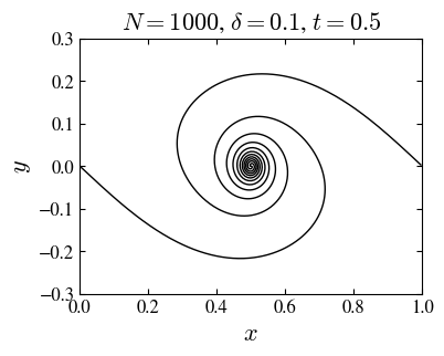
One may use the ode scipy integrator X = integrate.odeint(velocity, X0, t, args=(delta,)) to generate an array of point vortices $X = (x(t),y(t))$ trajectories, and plot it at different times (see figure).

Bifurcations

The nature of a fixed point $X$ can change at particular values of the parameters $a=a_*$, for instance a stable point becomes unstable. Changes of this kind, called bifurcations, are controled by the nonlinearities. Typical examples are the one dimensional dynamical systems depending on one parameter, such that the saddle-node bifurcation:

$$\dot{x} = a - x^2 \tag{SNb}$$

or the pitchfork bifurcation

$$\dot{x} = ax - x^3 \tag{Pb}$$

For the SNb there is no fixed point for $a<0$ and two fixed points for $a>0$, one stable ($x=\sqrt{a})$ and one unstable ($x=-\sqrt{a}$). The Pb describes instead the splitting of a stable fixed point $x=0$ for $a<0$, into two stable points $x=\pm\sqrt{a}$ for $a>0$. Increasing the dimension of the phase space and the parameter space lead to a rich variety of bifurcations. In two dimensions, one has for example the Hopf bifurcation that give rise to a limiting cycle:

$$\dot{r} = ar -r^3, \quad \dot{\theta} = 1 + br^2$$

in polar coordinates: for $a\le0$ the origin is a stable spiral (contracting algebraically if $a=0$), while for $a>0$, the circle $r=\sqrt{a}$ is attracting (limit cycle).

Example: Swift-Hohenberg equation

In the description of the convection of a fluid heated from below appears the Swift-Hohenberg equation, which describes the slow mode $u(x,y,t)$ of velocity field and thermal fields (noting the derivatives by indices):

$$u_t = ru - \big(\partial_x^2 + 1\big)^2 u - u^3 \tag{SH}\,,$$

where $r$ is the bifurcation parameter. The linear dispersion relation,

$$\sigma(k) = r - (k^2 - 1)^2\,,$$

describes the Rayleigh-Bénard instability of tha stable solution $u=0$ for $r<0$ to an unstable one for $r>0$, analogous to the pitchfork bifurcation. The amplitude of the unstable modes will obviously increase exponentially with a rate $\sigma(k)$, but they will also possess a spatial structure, given by any stationary solution of SH.

In one dimension, for $r>0$ the growth of an unstable mode can be described by

$$u(x,t) = \E^{\sigma t} f(x),\quad rf(x) = (\partial_x^2 +1)^2f(x)\,,$$

at the critical point $r=0$ we can take the $k=1$ mode:

$$u(x,t) = \cos(x)\,, \quad \sigma = 0\,,$$

which gives a spatially periodic pattern. A perturbation of this periodic pattern, after a transitory of exponential growth, will saturate to some asymptotic value: indeed, for large $u$ the nonlinear term cannot be neglected. To analyze the saturation at the critical point, we assume that the asymptotic solution has the same periodicity as the initial field:

$$u(x) = A \cos(x)\,.$$

Substituting into SH, and neglecting high order terms in $r$ and higher spatial harmonics ($k=3$, etc.), one readily obtains:

$$A = \sqrt{\frac{4r}{3}}$$

which is the saturation amplitude of the one dimensional spatially periodic solution with wavenumber $k=1$.

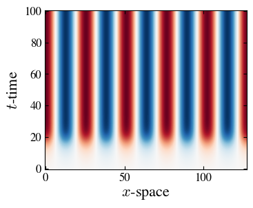
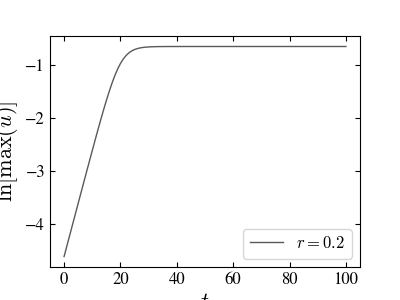
The above figure show the spatio-temporal diagram $u(x,t)$, and the growth of the amplitude in a log plot. The exponential growth and the subsequent saturation are well reproduced, the saturation amplitude $\max(u) = 0.561$ coincides with the theoretical prediction given by pitchfork bifurcation mechanism.

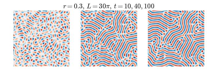
In two dimensions one can readily generalize the analysis taking $k_y=0$, which transforms the periodic one dimensional pattern in a series of parallel strips in the plane. However, other kind of instabilities arise, such as for instance a zig-zag one that ultimately will destroy the strips. The figure shows the evolution of an initially random field. The system tends to form strip domains, where the strips are differently oriented; the size of the domains growth with time (coarse-graining).

Numerics

We describe a numerical algorithm to integrate in time, a first order equation with, in general, linear and nonlinear terms:

$$u_t = Lu + NL(u,t),$$

where $L$ is a linear operator ($L = r - (\partial_{xx} + 1)$, for the SH equation) in and $NL$ the nonlinear part ($-u^3$ in SH). An implicit solution is obtained by integration,

$$u(t+h) = e^{Lh} u(t) + e^{Lh} \int_0^h dt' e^{-Lt'} NL(u,t')$$

Using the mid-point formula for the integral, one obtains the approximation method:

$$u(t+h) = e^{Lh} u(t) + \frac{e^{Lh}-1}{2L} \big[NL(u,t+h) + NL(u,t)\big]$$

which can be transformed in the predictor-corrector method,

$$u' = e^{Lh} u(t) + \frac{e^{Lh}-1}{L} NL(u,t)$$

and

$$u(t+h) = e^{Lh} u(t) + \frac{e^{Lh}-1}{2L} \big[NL(u',t+h) + NL(u,t)\big]$$

The spatial integration can easily be implemented using a pseudo-spectral algorithm: computing derivatives in fourier space and nonlinearities in real space.

#
# Swift-Hohenberg equation
# pseudo-spectral method with integrating factor

from scipy import fft
#
# parameters
r = 0.2
N = 128
T = 100
L  = 10*pi

k = 2.0*pi*fftfreq(N, L/N)
dt = 0.01
NT = int(T/dt)
ND = int(1/dt)
D = int(NT/ND) + 1
#
# integrating factor
LL = r - (-k**2 + 1)**2

E = exp(dt*LL)
EF = expm1(dt*LL)/LL
#
# initialize
dx = L/N
x  = dx*arange(N)

u0 = zeros(N)
u = zeros((D,N))
fu0 = zeros(N)
fu1 = zeros(N)
#
u0 = 0.01*cos(x)
u[0,:] = u0
fu0 = fft(u0)
#
# time evolution
it = 0
for t in arange(1,NT+1):
    Nfu0 = -fft(real(ifft(fu0))**3)
    fu1 = E*fu0 + EF*Nfu0

    Nfu1 = -fft(real(ifft(fu1))**3)
    fu0 = E*fu0 + 0.5*EF*(Nfu0 + Nfu1)
      if t%ND==0:
          it += 1
          u[it,:] = real(ifft(fu0))

Attractors

The long time behavior of dissipative systems is characterized by the contraction of the phase space volume, which tends to an asymptotic invariant set. A trivial example is given by the diffusion equation: an initial bounded concentration $c(x,0)$ evolves towards a uniform distribution $c(x,t)\rightarrow0$. This invariant set is an attractor and the set of initial conditions converging to the attractor is its basin of attraction. The dimension of the phase space attracting set is smaller than the phase space dimension. For instance the set $x(0)>0$ will converge to the set $x=1$ if $\dot{x} = x - x^3$, and the set $x(0)<1$ to $x=-1$, $t\rightarrow\infty$.

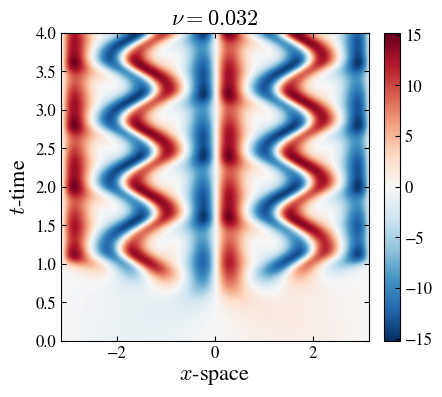
Kuramoto-Sivashinky equation

The Kuramoto-Sivashisky equation appears in the study of reaction diffusion fronts, and is a model of spatio-temporal chaos. It can be obtained from the Ginzburg-Landau equation, which governs the evolution of a superfluid, as an effective equation for the phase of the complex order parameter. In one dimension, and using convenient units, it reads,

$$u_t + uu_x + u_{xx} + u_{xxxx} = 0, \quad x \in [-L/2,L/2] \tag{KS}$$

(as before, indexes are for derivatives), where $u$ is related with the shape of the front (the displacement of the front with respect to a straight line). The only parameter of the system is its (nondimensional) size $L$. Using a simple scaling transformation on can also write (KS) with a (nondimensional) viscosity parameter $nu$:

$$u_t + uu_x + u_{xx} + \nu u_{xxxx} = 0, \quad x \in [-\pi,\pi] \tag{KSn}$$

with $L=2\pi/\sqrt{\nu}$.



Transition to spatio-temporal chaos in the Kuramoto-Shivashinsky equation.

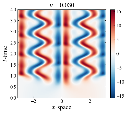
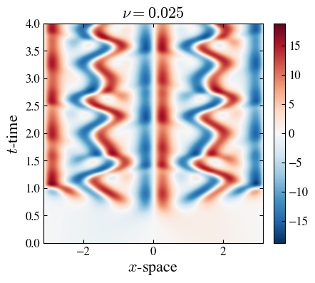
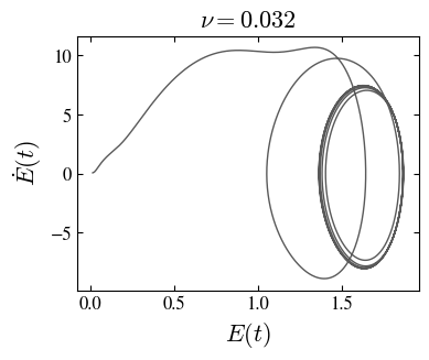
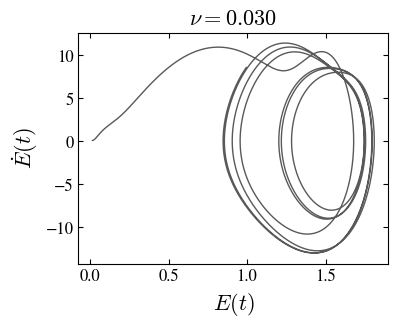
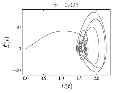
Varying the parameter $\nu$ from large values to small ones one observes transitions between different spatial and temporal patterns, form ordered to chaotic (Smyrlis and Papageorgiou, 1991). For instance arround $\nu = 0.03$ the system undergoes a series of period doubling bifurcations, similar to the Feigenbaum logistic map, leading to spatio-temporal chaos (figure above).

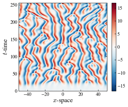
For smaller viscosity, or equivalently, when the system’s size increases, a regime of spatio-temporal chaos prevails; it is characterized by the power spectrum,

$$S(k) = \langle | u_k(t) |^2 \rangle$$

where the averaging is over time in the stationary regime. An estimation of the value of the threshold for disorder is given by the size of the most instable mode $L \sim 2\pi \sqrt{2} \approx 9$. The figure below show that the large length spectrum is flat, meaning an equipartition of the energy; there is a peak around $k \sim 1/\sqrt{2}$, followed by a power law region $S(k) \sim k^{-4}$, and finally, an exponential cutoff.


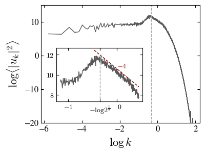Spatio-temporal chaos and its spectrum $S(k)$. The inset shows the unstable wavenumber region with an interval following a power law in $S(k) \sim k^{-4}$.

In summary the spectrum has the form,

$$S(k) \sim \frac{\E^{-k/k_\nu}}{k^4}$$

where $k_\nu$ is the viscous cutoff.

Lorenz system

The Lorenz system results from a truncation of the hydrodynamic fluid equations describing thermal convection in a slab geometry. The velocity and temperature fields are truncated to three fourier amplitudes $(x,y,z)$, satisfying the set of ordinary differential equations:

\begin{align*} \dot{x} &= s(y-x)\\ \dot{y} &= r x - y - xz\\ \dot{z} &= -bz + xy \end{align*}

depending on the parameter set $(s,r,b)$ related to the Prandtl number $\mathrm{Pr}$, the Rayleigh number $\mathrm{Ra}$ and a characteristic length of the convective rolls, respectively.

The code below is a python implementation of the Lorenz system:

from numpy import *
from matplotlib.pyplot import *
from scipy import integrate
from mpl_toolkits.mplot3d import Axes3D
# Lorenz attractor
#
def lorenz(X, t, a):
    s, r, b = a
    x, y, z = (X[0], X[1], X[2])
    dx = s*(y - x)
    dy = r*x - x*z - y
    dz = x*y - b*z
    return [dx, dy, dz]
#
X0 = [1, 1, 1] # initial condition
t = linspace(0, 40, 5000) # time steps
a = (10, 28, 8/3) # (s, r, b)
#
# phase space trajectory X(t), shape(X) = (t,3)
X = integrate.odeint(lorenz, X0, t, args=(a,))
fig = figure(figsize = (6,6))
ax = fig.add_subplot(111, projection='3d')
plot(X[:,0], X[:,1], X[:,2])
show()

The program returns a plot of the trajectory in the phase space, for the case $s=10$, $r=28$ and $b =8/3$ first used by Lorenz.

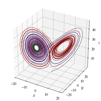
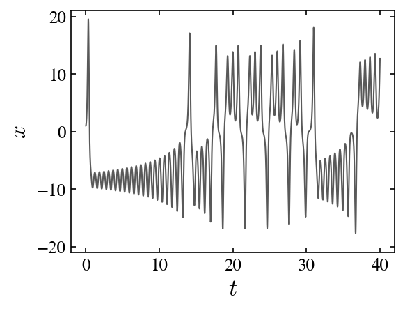
The figure above shows the phase-space trajectory $\boldsymbol{X}(t)$, $\boldsymbol{X} = (x,y,z)$, for a time spaning the interval $t \in (0,T=40)$, with different colors for $t < 0.2T$ (black), $0.2T<t<0.5T$ (blue) and $t>0.5T$ (red), to underline the structure of the attractor. It consists in two lobes, and the trajectory intermittently switch from one to the other, as can be seen in the plot $x = x(t)$.

Strange attractor

Under the dynamics $\dot{\boldsymbol{X}} = \boldsymbol{F}(\boldsymbol{X})$ the phase-space volume $V$ shrinks exponentially:

$$\frac{\D}{\D t}V(t) = \int \D V\, \nabla \cdot \boldsymbol F = -(s+1+b)V\,,$$

which implies that the attractor set has measure zero in the three dimensional phase-space. It is an example of strange attractor.

Hydrodynamic equations

We consider a vertical layer $(x,y)$ of fluid of height $h$, $y \in (0,h)$, subject to a temperature gradient $(T_h - T_0)/h <0$. To simplify the analysis we assume homogeneity in the horizonatal $z$-direction, $\nabla = (\partial_x,\partial_y,0)$. The fluid velocity $\boldsymbol{v}$ and the temperature $T$, satisfy,

$$\rho\left( \frac{\partial }{\partial t} \boldsymbol v + \boldsymbol v \cdot \nabla \boldsymbol v \right) = -\nabla p - \rho g \hat{\boldsymbol y} + \mu \nabla^2 \boldsymbol v\,,$$

where $\mu$ is the viscosity, and

$$\frac{\partial }{\partial t} T + \boldsymbol v \cdot \nabla T = D \nabla^2 T\,,$$

where $D$ is the thermal diffusivity. The temperature variation $\Delta T$ induces a density variation $\rho = \rho(T)$, characterized by the dilatation coefficient $\alpha$:

$$\Delta \rho = -\rho_0 \alpha \Delta T\,,\quad \alpha = - \frac{1}{\rho_0} \frac{\partial \rho}{\partial T}\,.$$

The equilibrium solution of these equations is

$$\boldsymbol v = 0,\; T_0(y) = T_0 + \frac{T_h - T_0}{h} y = T_0 - \frac{\delta T}{h}y, \; \frac{\D p_0(y)}{\D y} = -g\rho_0(y,T) \,,$$

where $\delta T = T_0 - T_h > 0$. Using

$$\rho_0(y,T) = \rho_0 + \rho_0 \alpha \frac{\delta T}{h} y,$$

we obtain,

$$p_0(y) = p_0 - \rho_0 g y - \rho_0 \alpha \frac{\delta T}{2h} y^2.$$

Fluctuations $\boldsymbol v$, $\Delta T = T - T_0(y)$ and $\Delta p=p - p_0(y)$, once substituted into the hydrodynamic equations, satisfy,

$$\rho_0\left( \frac{\partial }{\partial t} \boldsymbol v + \boldsymbol v \cdot \nabla \boldsymbol v \right) = -\nabla \Delta p + \rho_0 \alpha g \Delta T \hat{\boldsymbol y} + \mu \nabla^2 \boldsymbol v\,,$$

where we neglegted variations of the density in the left hand side, and

$$\frac{\partial }{\partial t} \Delta T + \boldsymbol v \cdot \nabla \Delta T + v_y \frac{\delta T}{h} = D \nabla^2 \Delta T\,.$$

Now, introducing the units of length $h$, time $h^2/D$, density $\rho_0$ and temperature $\delta T$, and dropping the $\Delta$ notation for the fluctuations, we finally obtain

$$\frac{1}{\mathrm{Pr}}\left(\frac{\partial }{\partial t} \boldsymbol v + \boldsymbol v \cdot \nabla \boldsymbol v \right)= -\nabla p + \mathrm{Ra} T \hat{\boldsymbol z} + \nabla^2 \boldsymbol v\,,$$

and

$$\frac{\partial }{\partial t} T + \boldsymbol v \cdot \nabla T + v_y = \nabla^2 T\,,$$

in adimensional form, where

$$\mathrm{Ra} = \frac{\rho_0 g h^3 \alpha \delta T}{D\mu},\; \mathrm{Pr} = \frac{\mu}{\rho_0 D}$$

are the Rayleigh and Prandtl numbers, respectively.

Introducing the stream function $\psi$:

$$v_x=\frac{\partial }{\partial y}\psi,\; v_y=-\frac{\partial }{\partial x}\psi\,,$$

and taking the rotational of the velocity equation to eliminate the pressure gradient, we obtain,

$$\frac{1}{\mathrm{Pr}}\left(\frac{\partial }{\partial t} \nabla^2 \psi + [\psi, \nabla^2 \psi]\right) = \mathrm{Ra} \frac{\partial T}{\partial x} + \nabla^4 \psi$$

and

$$\frac{\partial }{\partial t}T + [\psi,T] - \frac{\partial }{\partial x}\psi = \nabla^2 T,,$$

where $[\ldots]$ is the Poisson bracket:

$$[f,g]= \frac{\partial f}{\partial x} \frac{\partial g}{\partial y} - \frac{\partial f}{\partial y} \frac{\partial g}{\partial x}\,.$$

The Lorenz system results from the Ansatz,

\begin{align*} \psi(x,y,t) &= p(t) \sin(kx) \sin(\pi y)\\ T(x,y,t) &= a(t) \cos(kx) \sin(\pi y) - b(t) \sin(2\pi y) \end{align*}

We may use sympy to deduce the differential equations in the amplitudes $(p,a,b)$.

from sympy import *

s, r, k = symbols('s, r, k', reals = True, positive = True)
x, y, t = symbols('x, y, t', reals = True)
#
p = Function('p') # psi amplitude
a = Function('a') # temperature amplitude
b = Function('b') # temperature amplitude
#
# Ansatz
psi = p(t)*sin(k*x)*sin(pi*y)
T = a(t)*cos(k*x)*sin(pi*y) - b(t)*sin(2*pi*y)
#
def Dt(f):
    return f.diff(t)
def Dx(f):
    return f.diff(x)
def Dy(f):
    return f.diff(y)
def Lap(f):
    return f.diff(x,2) + f.diff(y,2)
def Poisson(f, g):
    return f.diff(x)*g.diff(y) - f.diff(y)*g.diff(x)
#
# hydrodynamic equations
eq_temp = Dt(T) + Poisson(psi, T) - Dx(psi) - Lap(T)
eq_psi = Dt(Lap(psi)) + Poisson(psi, Lap(psi)) - r*s*Dx(T) - s*Lap(Lap(psi))

Simplification of the temperature equation: first collect the $\cos(kx)\sin(\pi y)$ terms, neglect the $\sin(3\pi y)$ term in the development of $\cos(2\pi y)\sin(\pi y)$, and finally collect $\sin(2\pi y)$ terms.

collect(trigsimp(collect(
        collect(
            expand(eq_temp).subs(cos(2*pi*y)*sin(pi*y),
            -Rational(1,2)*sin(pi*y)), 
        sin(pi*y)*cos(k*x)), 
    pi*k*a(t)*p(t))), sin(2*pi*y))
#
# Output:
(pi*k*a(t)*p(t)/2 - 4*pi**2*b(t) - Derivative(b(t), t))*sin(2*pi*y) +
(k**2*a(t) + pi*k*b(t)*p(t) - k*p(t) + pi**2*a(t) + Derivative(a(t), t))*
sin(pi*y)*cos(k*x)

Simplification of the stream function equation: collect terms in $\sin(kx)\sin(\pi y)$ and $p$.

simplify(collect(factor(simplify(eq_psi))/(sin(pi*y)*sin(k*x)), p(t)))
#
# Output:
k*r*s*a(t) - s*(k**4 + 2*pi**2*k**2 + pi**4)*p(t) -
(k**2 + pi**2)*Derivative(p(t), t)

Collecting the coefficients of the different trigonometric functions we arrive at,

\begin{align*} \dot{p} &= -(\pi^2 + k^2) p + \frac{k s r}{\pi^2 + k^2} a\\ \dot{a} &= -(\pi^2 + k^2) a + k p - \pi k b p\\ \dot{b} &= -4\pi^2 b + \frac{\pi k}{2} a p \end{align*}

which are, after rescaling, the Lorenz equations.

Bibliography

Strogatz, S. H. Nonlinear dynamics and chaos (CRC, 2015).
Cross, M. and Greenside, H. Pattern Formation (Cambridge, 2009). An interesting and thorough introduction to nonlinear dynamics and nonequilibrium systems.

»chaos »map »hamiltonian systems »plasmas